Bayesian Methods - Normal-gamma example

Full assignment in PDF

Send your solutions to: vavraj@karlin.mff.cuni.cz by 3 November, 9:00

Normal-gamma example

When measuring the speed of \(n = 50\) cars on Rohanské nábřeží, opposite of the MFF building, we obtained the sample mean \(\overline y = 59.6\) and the sample standard deviation of \(s = 11.1\) km/h (the measurements were taken in the period before installation of two traffic lights at the corners of the River Garden office building).

Examine the posterior distribution of the mean (expected value) of the speed of cars at Rohanské nábřeží while assuming a normal distribution \(\mathsf{N}(\mu,\sigma^2)\) of the speed. As a prior for \(\mu\) and \(\tau = \sigma^{-2}\) consider a (semi-conjugate) distribution: \[ p(\mu,\,\tau) = p(\mu)\,p(\tau), \] where \(p(\mu) \propto 1\) and \(\tau\sim\mathsf{\Gamma}(g,\,h)\), \(p(\tau) \propto \tau^{g-1}\exp(-\,h\,\tau)\). For \(g\) and \(h\) consider the following choices:

1. \(g = 0.001\), \(h = 0.001\);
2. \(g = 1\), \(h = 0.005\);
3. \(g = 0\), \(h = 0\) (improper distribution with \(p(\tau) \propto \tau^{-1}\)).

n <- 50 
Yhat <- 59.6 # km/h
sdhat <- 11.1 # km/h

alpha <- 0.05

g <- c(0.001, 1, 0)
h <- c(0.001, 0.005, 0)

Task 1 - Frequentistic approach

As a check, calculate the ordinary (i.e., non-bayesian, frequentist) 95% confidence interval for the unknown mean \(\mu\) and also for the standard deviation \(\sigma\) and inverse variance \(\tau\).

We can derive the CI from the following distributions: \[ \overline{Y}_n \sim \mathsf{N}\left(\mu,\, \frac{\sigma^2}{n}\right) \qquad \text{and} \qquad \frac{(n-1)S_n^2}{\sigma^2} \sim \chi_{n-1}^2. \]

CI <- list()
CI$mu <- CI$tau <- CI$sigma <- list()

(CI$mu$Freq <- Yhat + c(-1,1)*qt(1-alpha/2,df=n-1)*sdhat/sqrt(n))

## [1] 56.44541 62.75459

chi_quantiles <- qchisq(c(alpha/2,1-alpha/2),df=n-1)
(CI$sigma$Freq <- sdhat*sqrt((n-1)/rev(chi_quantiles)))

## [1]  9.272208 13.832080

(CI$tau$Freq <- chi_quantiles/(sdhat^2*(n-1)))

## [1] 0.005226669 0.011631446

Task 2 - Marginal posterior distribution of \(\mu\)

Derive the marginal posterior distribution for \(\mu\) and plot its density (in one figure) for the above choices \(g\) and \(h\). What is the posterior probability that the mean of the speed is greater than 55 km/h (again for three different choices of \(g\) and \(h\))?

We need to marginalize the following pdf with respect to \(\tau\):

\[ p(\mu, \tau | \mathbb{Y}) \propto p(\mathbb{Y} | \mu, \tau) p(\mu, \tau) \propto \tau^{\frac{n}{2}} \exp \left\{-\frac{\tau}{2}\sum\limits_{i=1}^n(Y_i - \mu)^2\right\} \cdot 1 \cdot \tau^{g-1} \exp \left\{-\tau h\right\}. \] This envolves integration \(\int\limits_{0}^\infty \cdots \mathrm{d}\tau\), which can be solved by using knowledge of \(\Gamma(\alpha, \lambda)\) distribution.

Hint: Up to a multiplicative constant, you should recognize the remaining function of \(\mu\) as pdf of Location-scale Student distribution.

mu.grid <- seq(CI$mu$Freq[1] - 0.3*diff(range(CI$mu$Freq)),
               CI$mu$Freq[2] + 0.3*diff(range(CI$mu$Freq)), 
               length.out = 101)

dpost_mu <- function(x, g=0, h=0){
  a <- sqrt((2*h+(n-1)*sdhat^2)/(n*(n+2*g-1)))
  d <- dt((x-Yhat)/a, df = n+2*g-1) / a
  return(d)
}
ppost_mu <- function(x, g=0, h=0){
  a <- sqrt((2*h+(n-1)*sdhat^2)/(n*(n+2*g-1)))
  p <- pt((x-Yhat)/a, df = n+2*g-1)
  return(p)
}

dens_mu <- apply(cbind(g,h), 1, function(gh){
  dpost_mu(mu.grid, g = gh["g"], h = gh["h"])
})

prst.mu.nad.55 <- apply(cbind(g,h), 1, function(gh){
  1 - ppost_mu(55, g = gh["g"], h = gh["h"])
})


LWD <- c(2,2,4)
LTY <- c(1,2,3)
COL <- c("darkorange", "red3", "blue")

par(mfrow = c(1,1), mar = c(4,4,2.5,0.5))
plot(rep(0, length(mu.grid)) ~ mu.grid, type = "n",
     xlab = "Car speed [km/h]", ylab = "Density",
     main = expression("Marginal posterior density of" ~ mu),
     ylim = range(dens_mu), xlim = range(mu.grid))
for(i in 1:3){
  lines(mu.grid, dens_mu[,i], col = COL[i], lty = LTY[i], lwd = LWD[i])
}
abline(v=Yhat, col = "darkgrey", lty = 2, lwd=2)
abline(v=55, col = "darkorchid", lty = 5, lwd=1)
abline(v=CI$mu$Freq, col = "yellowgreen", lty = 3, lwd=1)
text(x = Yhat, y = 0.1*max(dens_mu), pos = 4,
     eval(substitute(expression(paste(hat(mu), " = ", Yhat, sep="")),
                     list(Yhat = round(Yhat, digits =2)))))
legend("topright", legend = paste0("g=",g,"\nh=",h),
       col = COL, lty = LTY, lwd = LWD, bty = "n", y.intersp = 2)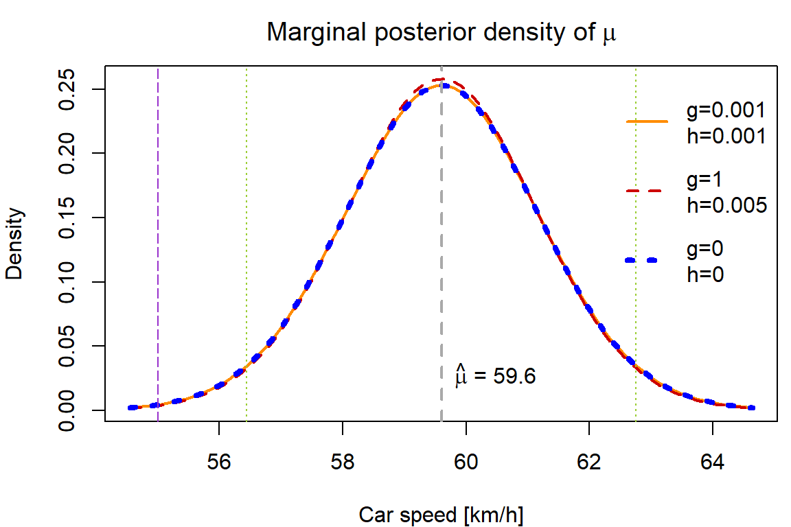

Task 3 - Marginal posterior distribution of \(\mu\)

Derive the marginal posterior distribution for \(\tau\) and plot its density (in one figure) for the above choices \(g\) and \(h\). In the second plot, draw the marginal posterior densities for \(\sigma = \sqrt{1/\tau}\). Note that it is not necessary to explicitly derive the formula for the posterior density of \(\sigma\) for the purpose of plotting once you have a computer function to calculate the functional values of the posterior density of \(\tau\).

We need to marginalize the following pdf with respect to \(\mu\):

\[ p(\mu, \tau | \mathbb{Y}) \propto p(\mathbb{Y} | \mu, \tau) p(\mu, \tau) \propto \tau^{\frac{n}{2}+g-1} \exp \left\{-\tau \left[\frac{1}{2}\sum\limits_{i=1}^n(Y_i - \mu)^2 + h\right]\right\}. \] This envolves integration \(\int\limits_{-\infty}^\infty \cdots \mathrm{d}\mu\), which can be solved by using knowledge of \(\mathsf{N}(\mu,\sigma^2)\) distribution.

Hints: Up to a multiplicative constant, you should recognize the remaining function of \(\tau\) as pdf of some well known distribution. To obtain the marginal posterior density of \(\sigma\) use transformation theorem.

tau.grid <- seq(CI$tau$Freq[1]-0.2*diff(range(CI$tau$Freq)),
                CI$tau$Freq[2]+0.4*diff(range(CI$tau$Freq)), 
                length.out = 101)
tauhat <- 1/sdhat^2

dens_tau <- apply(cbind(g,h), 1, function(gh){
  dgamma(tau.grid, shape = (n-1)/2+gh["g"], rate = sdhat^2*(n-1)/2 + gh["h"])
})

sigma.grid <- seq(CI$sigma$Freq[1]-0.2*diff(range(CI$sigma$Freq)),
                  CI$sigma$Freq[2]+0.4*diff(range(CI$sigma$Freq)), 
                  length.out = 101)
dens_sigma <- apply(cbind(g,h), 1, function(gh){
  2/sigma.grid^3 * dgamma(1/sigma.grid^2, shape = (n-1)/2+gh["g"], rate = sdhat^2*(n-1)/2 + gh["h"])
})

par(mfrow = c(1,2), mar = c(4,4,2.5,0.5))
# tau
plot(rep(0, length(tau.grid))~tau.grid, type = "n",
     xlab = expression(tau), ylab = "Density",
     main = expression("Marginal posterior density of " ~ tau),
     ylim = range(dens_tau))
for(i in 1:3){
  lines(tau.grid, dens_tau[,i], col = COL[i], lty = LTY[i], lwd = LWD[i])
}
abline(v=tauhat, col = "darkgrey", lty = 2, lwd = 2)
abline(v=CI$tau$Freq, col = "yellowgreen", lty = 3, lwd=1)
text(x = tauhat, y = 0.1*max(dens_tau), pos = 4,
     eval(substitute(expression(paste(hat(tau), " = ", tauhat, sep="")),
                     list(tauhat = round(tauhat, digits =5)))))
legend("topright", legend = c("g=0.001\nh=0.001",
                             "g=1\nh=0.001", 
                             "g=h=0"),
       col = COL, lwd = LWD, lty = LTY, bty = "n", y.intersp = 2)

# sigma
plot(rep(0, length(sigma.grid))~sigma.grid, type = "n",
     xlab = expression(sigma), ylab = "Density",
     main = expression("Marginal posterior density of " ~ sigma),
     ylim = range(dens_sigma))
for(i in 1:3){
  lines(sigma.grid, dens_sigma[,i], col = COL[i], lty = LTY[i], lwd = LWD[i])
}
abline(v=sdhat, col = "darkgrey", lty = 2, lwd=2)
abline(v=CI$sigma$Freq, col = "yellowgreen", lty = 3, lwd=1)
text(x = sdhat, y = 0.1*max(dens_sigma), pos = 4,
     eval(substitute(expression(paste(hat(sigma), " = ", sdhat, sep="")),
                     list(sdhat = round(sdhat, digits =5)))))

legend("topright", legend = paste0("g=",g,"\nh=",h),
       col = COL, lwd = LWD, lty = LTY, bty = "n", y.intersp = 2)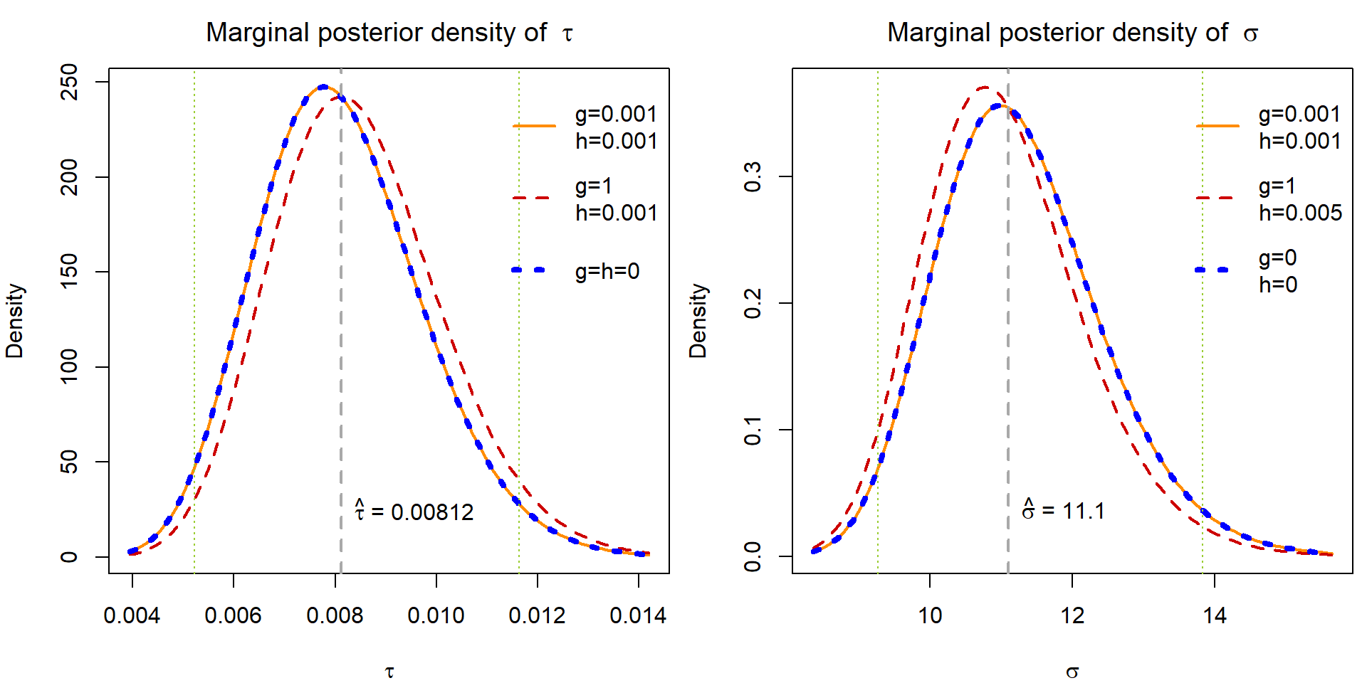

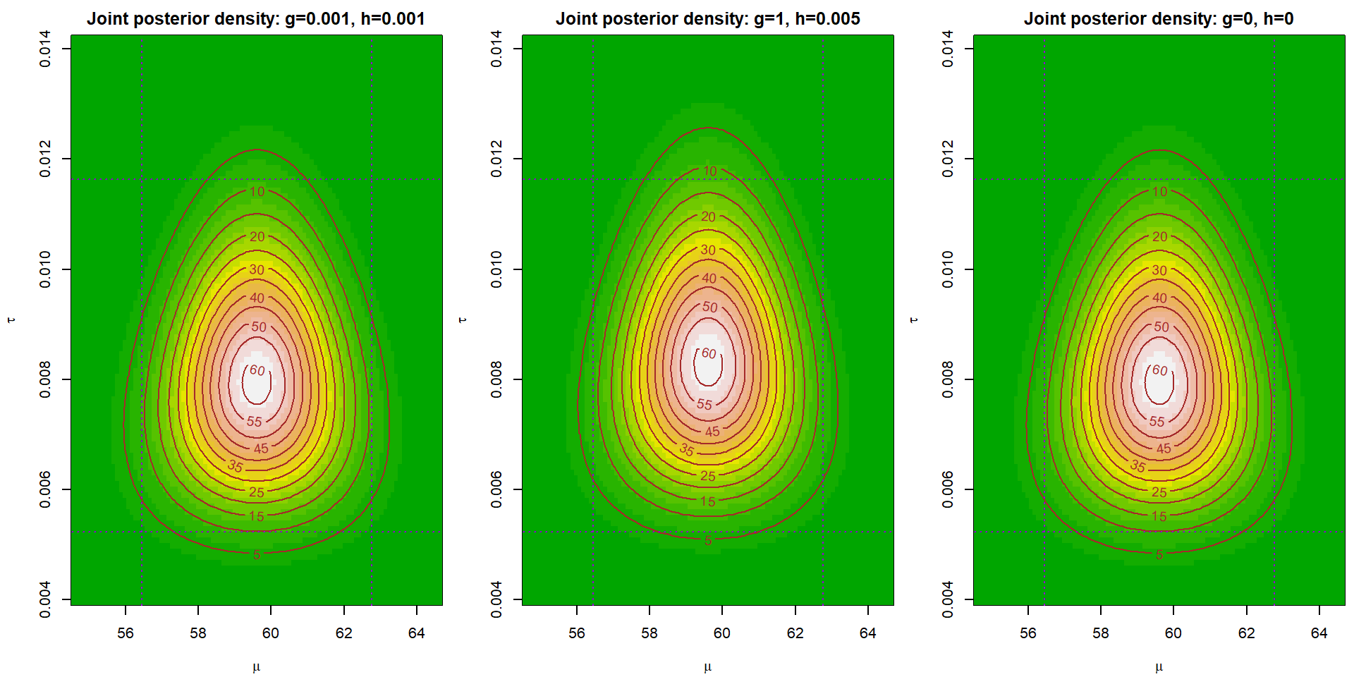
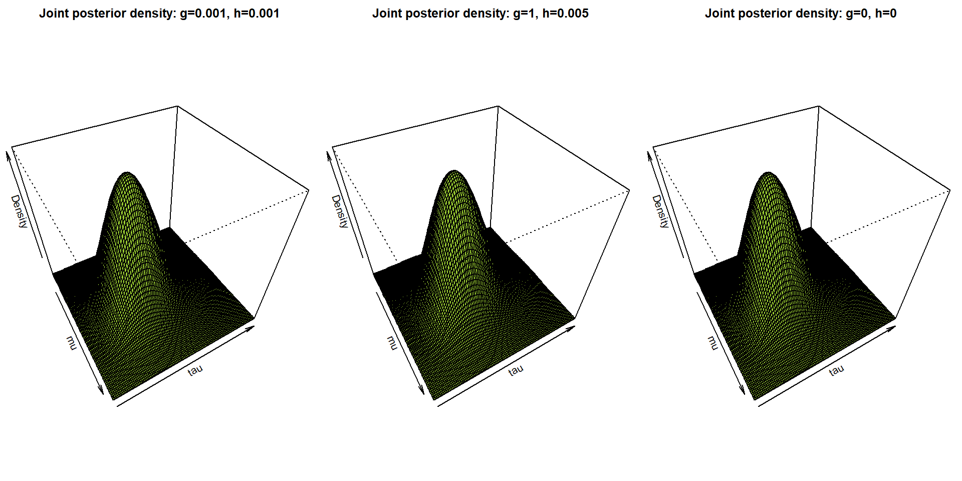
Task 4 - Joint posterior density of \((\mu,\,\tau)\)

Draw (in three different plots) plot of a joint posterior density of \((\mu,\,\tau)\) for three different choices of \(g\) and \(h\). Note that you can use the relation \(p(\mu,\,\tau\,|\,\mathbb{Y}) = p(\mu,\,\tau\,|\,\mathbb{Y})\,p(\tau\,|\,\mathbb{Y})\) to calculate the functional values of \(p(\mu,\,\,\tau\,|\,\mathbb{Y})\).

Hint: Use the following functions:

x; y                         # grids on x and y axis
z <- outer(x, y, fun)        # fun = function of x and y to be evaluated
image(x, y, z)               # creates colourful plot
contour(x, y, z, add = T)    # adds contours 
# alternatively
persp(x, y, z)               # 3D plot

mutau_posterior <- function(mu, tau, g = 0, h = 0){
  dtau <- dgamma(tau, shape = (n-1)/2+g, rate = sdhat^2*(n-1)/2 + h)
  dmu_tau <- dnorm(mu, mean = Yhat, sd = 1/sqrt(tau*n))
  return(dtau * dmu_tau)
}

mutau_dens <- list()
for(i in 1:3){
  mutau_dens[[i]] <- outer(mu.grid, tau.grid, mutau_posterior, g = g[i], h = h[i])
}

par(mfrow = c(1,3), mar = c(4,4,2,0.5))
for(i in 1:3){
  image(mu.grid, tau.grid, mutau_dens[[i]], col = terrain.colors(20),
        xlab = expression(mu), ylab = expression(tau), 
        zlim = range(mutau_dens),                                       # common scale for all three plots
        main = paste0("Joint posterior density: g=",g[i],", h=",h[i]))
  contour(mu.grid, tau.grid, mutau_dens[[i]], col="brown", add=TRUE)
  abline(v = CI$mu$Freq, col = "darkviolet", lty = 3, lwd = 1)
  abline(h = CI$tau$Freq, col = "darkviolet", lty = 3, lwd = 1)
}

par(mfrow = c(1,3), mar = c(0,0,2,0))
for(i in 1:3){
  persp(mu.grid, tau.grid, mutau_dens[[i]], col = "yellowgreen",
        xlab = expression(mu), ylab = expression(tau), zlab = "Density",
        zlim = range(mutau_dens),                                       # common scale for all three plots
        theta = 60, phi = 45,
        main = paste0("Joint posterior density: g=",g[i],", h=",h[i]))
}

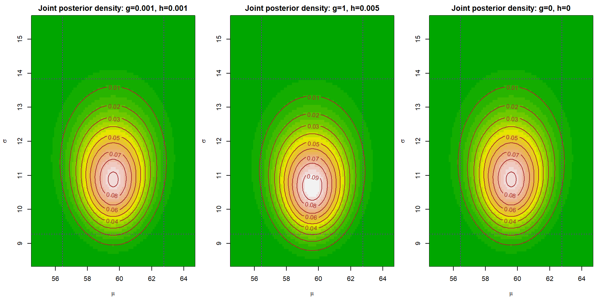
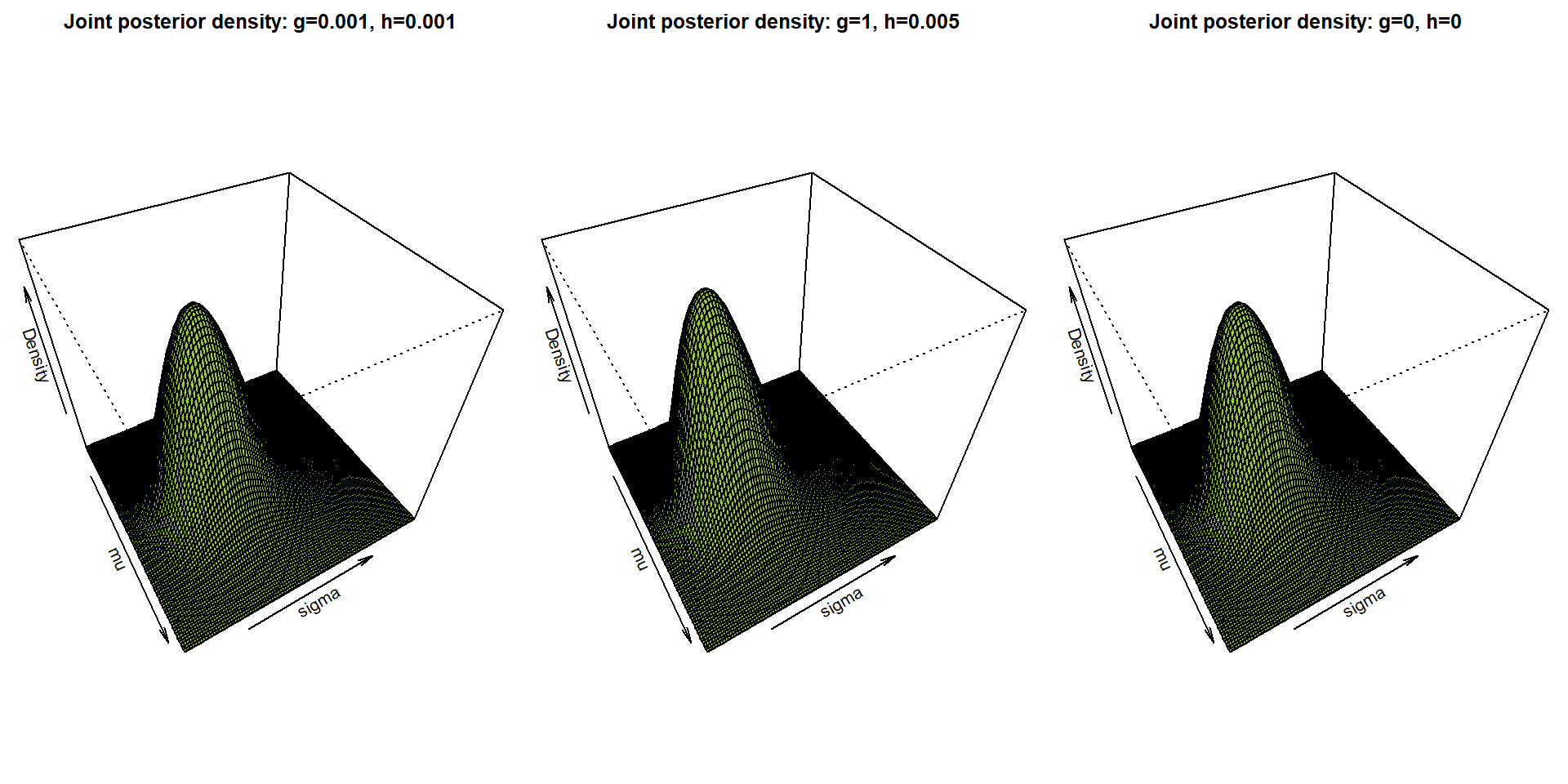
Task 5 - Joint posterior density of \((\mu,\,\sigma)\)

Draw (in three different plots) plot of a joint posterior density of \((\mu,\,\sigma)\) for three different choices of \(g\) and \(h\). Note that you can use the relation \(p(\mu,\,\sigma\,|\,\mathbb{Y}) = p(\mu,\,\sigma\,|\,\mathbb{Y})\,p(\sigma\,|\,\mathbb{Y})\) to calculate the functional values of \(p(\mu,\,\,\sigma\,|\,\mathbb{Y})\). Moreover, \(p(\mu\,|\,\sigma,\,\mathbb{Y}) = p\bigl(\mu\,\big|\,\sigma^{-2},\,\mathbb{Y}\bigr)\).

musigma_posterior <- function(mu, sigma, g = 0, h = 0){
  dsigma <- 2/sigma^3 * dgamma(1/sigma^2, shape = (n-1)/2+g, rate = sdhat^2*(n-1)/2 + h)
  dmu_sigma <- dnorm(mu, mean = Yhat, sd = sigma/sqrt(n))
  return(dsigma * dmu_sigma)
}

musigma_dens <- list()
for(i in 1:3){
  musigma_dens[[i]] <- outer(mu.grid, sigma.grid, musigma_posterior, g = g[i], h = h[i])
}

par(mfrow = c(1,3), mar = c(4,4,2,0.5))
for(i in 1:3){
  image(mu.grid, sigma.grid, musigma_dens[[i]], col = terrain.colors(20),
        xlab = expression(mu), ylab = expression(sigma), 
        zlim = range(musigma_dens),                                       # common scale for all three plots
        main = paste0("Joint posterior density: g=",g[i],", h=",h[i]))
  contour(mu.grid, sigma.grid, musigma_dens[[i]], col="brown", add=TRUE)
  abline(v = CI$mu$Freq, col = "darkviolet", lty = 3, lwd = 1)
  abline(h = CI$sigma$Freq, col = "darkviolet", lty = 3, lwd = 1)
}

par(mfrow = c(1,3), mar = c(0,0,2,0))
for(i in 1:3){
  persp(mu.grid, sigma.grid, musigma_dens[[i]], col = "yellowgreen",
        xlab = expression(mu), ylab = expression(sigma), zlab = "Density",
        zlim = range(musigma_dens),                                       # common scale for all three plots
        theta = 60, phi = 45,
        main = paste0("Joint posterior density: g=",g[i],", h=",h[i]))
}

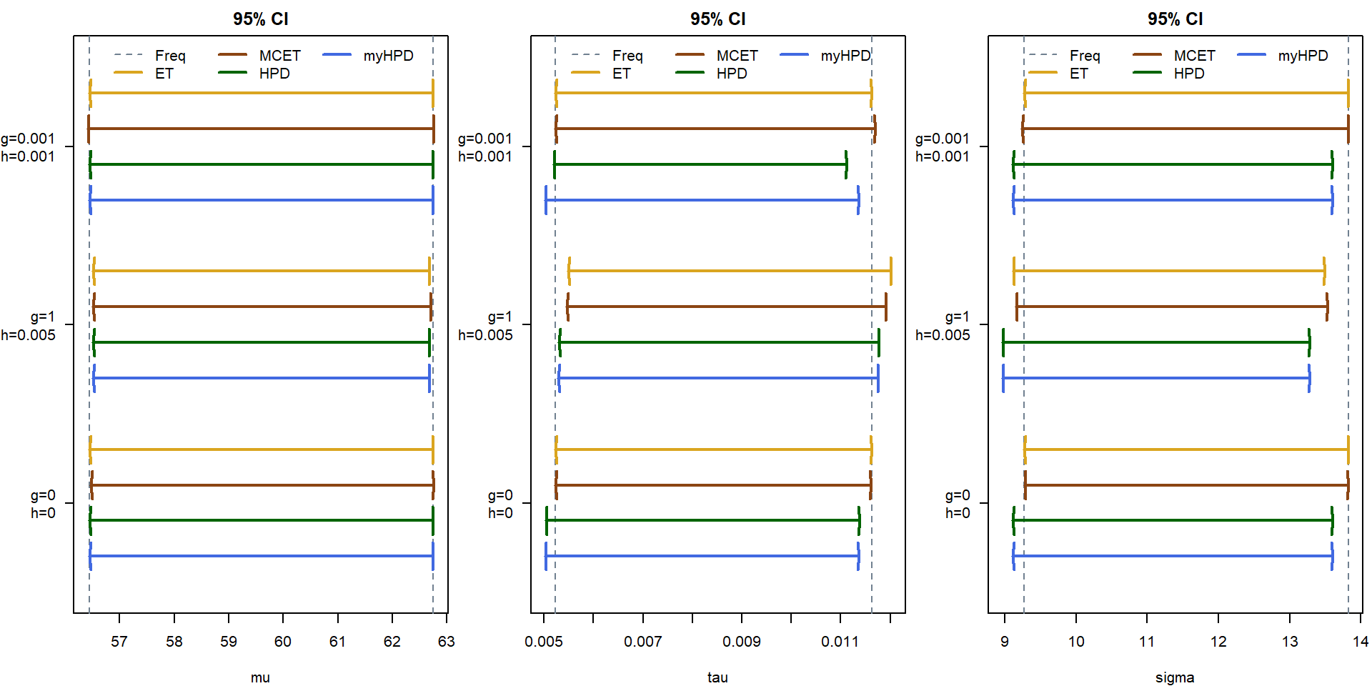
Task 6 - Equal-tail (ET) credible intervals

Calculate the 95% ET (equal-tail) credible interval for \(\mu\), \(\tau\), \(\sigma\) and each choice of \(g\) and \(h\).

CI$mu$ET <- CI$tau$ET <- CI$sigma$ET <- matrix(0,3,2)
for (i in 1:3){
  a <- sqrt((2*h[i]+(n-1)*sdhat^2)/(n*(n+2*g[i]-1)))
  CI$mu$ET[i, ] <- Yhat + a*qt(c(alpha/2, 1-alpha/2), df = n+2*g[i]-1)
  CI$tau$ET[i, ] <- qgamma(c(alpha/2, 1-alpha/2), shape = (n-1)/2+g[i], rate = sdhat^2*(n-1)/2+h[i])
  CI$sigma$ET[i, ] <- rev(sqrt(1/CI$tau$ET[i,]))
}
colnames(CI$mu$ET) <- colnames(CI$tau$ET) <- colnames(CI$sigma$ET) <- c("Lower 95% ETCI", "Upper 95% ETCI")
CI$mu$ET

##      Lower 95% ETCI Upper 95% ETCI
## [1,]       56.44548       62.75452
## [2,]       56.51095       62.68905
## [3,]       56.44541       62.75459

CI$tau$ET

##      Lower 95% ETCI Upper 95% ETCI
## [1,]    0.005226933     0.01163184
## [2,]    0.005492817     0.01202789
## [3,]    0.005226669     0.01163145

CI$sigma$ET

##      Lower 95% ETCI Upper 95% ETCI
## [1,]       9.272051       13.83173
## [2,]       9.118119       13.49281
## [3,]       9.272208       13.83208

Task 7 - Highest posterior density (HPD) credible intervals

Calculate (numerically, if needed) the 95% HPD (highest posterior density) credible interval for \(\mu\), \(\tau\), \(\sigma\) and each choice of \(g\) and \(h\). Do those intervals differ from the ET credible intervals?

CI$mu$HPD <- CI$mu$ET # posterior for mu is symmetric
# posteriors of tau and sigma are NOT symmetric
CI$tau$HPD <- CI$sigma$HPD <- matrix(0,3,2)
for(i in 1:3){
  objF <- function(x){
    return(abs(pgamma(x[2], shape = (n-1)/2+g[i], rate = sdhat^2*(n-1)/2 + h[i]) -
               pgamma(x[1], shape = (n-1)/2+g[i], rate = sdhat^2*(n-1)/2 + h[i]) -1+alpha)+
           abs(dgamma(x[2], shape = (n-1)/2+g[i], rate = sdhat^2*(n-1)/2 + h[i]) -
               dgamma(x[1], shape = (n-1)/2+g[i], rate = sdhat^2*(n-1)/2 + h[i])))}
  #optim(par = CI$tau$ET[i,], fn = objF, method = "Nelder-Mead", control = list(maxit = 2000))
  #optim(par = CI$tau$ET[i,], fn = objF, method = "Nelder-Mead", control = list(maxit = 2000))
  #optim(par = CI$tau$ET[i,], fn = objF, method = "BFGS")
  #optim(par = CI$tau$ET[i,], fn = objF, method = "CG")
  #optim(par = CI$tau$ET[i,], fn = objF, method = "L-BFGS-B", lower = c(0.0005,0.0005), upper = c(0.1,0.1))
  #optim(par = CI$tau$Freq, fn = objF)
  vysl <- optim(par = c(tauhat-0.001,tauhat+0.001), fn = objF, control = list(maxit = 10000))
  CI$tau$HPD[i,] <- vysl$par
  # sigma 
  # CI$sigma$HPD[i,] <- rev(sqrt(1/CI$tau$HPD[i,]))
  objFsigma <- function(x){
    return(abs(pgamma(1/x[1]^2, shape = (n-1)/2+g[i], rate = sdhat^2*(n-1)/2 + h[i])-
               pgamma(1/x[2]^2, shape = (n-1)/2+g[i], rate = sdhat^2*(n-1)/2 + h[i])-1+alpha)+
       10*abs(2/x[1]^3*dgamma(1/x[1]^2, shape = (n-1)/2+g[i], rate = sdhat^2*(n-1)/2 + h[i])-
               2/x[2]^3*dgamma(1/x[2]^2, shape = (n-1)/2+g[i], rate = sdhat^2*(n-1)/2 + h[i])))}
  
  vysl <- optim(par = c(sdhat-1,sdhat+1), # CI$sigma$ET[i,], 
                fn = objFsigma, control = list(maxit = 10000))
  CI$sigma$HPD[i,] <- vysl$par
}
colnames(CI$mu$HPD) <- colnames(CI$tau$HPD) <- colnames(CI$sigma$HPD) <- 
  c("Lower 95% HPDCI", "Upper 95% HPDCI")

CI$tau$HPD

##      Lower 95% HPDCI Upper 95% HPDCI
## [1,]     0.005194652      0.01112050
## [2,]     0.005303683      0.01178139
## [3,]     0.005038244      0.01138449

1/sqrt(CI$tau$HPD)

##      Lower 95% HPDCI Upper 95% HPDCI
## [1,]        13.87464        9.482828
## [2,]        13.73129        9.213013
## [3,]        14.08836        9.372235

CI$sigma$HPD

##      Lower 95% HPDCI Upper 95% HPDCI
## [1,]        9.112482        13.60807
## [2,]        8.967318        13.28291
## [3,]        9.112630        13.60840

all.equal(CI$tau$ET, CI$tau$HPD)

## [1] "Attributes: < Component \"dimnames\": Component 2: 2 string mismatches >"
## [2] "Mean relative difference: 0.02760932"

all.equal(CI$sigma$ET, CI$sigma$HPD)

## [1] "Attributes: < Component \"dimnames\": Component 2: 2 string mismatches >"
## [2] "Mean relative difference: 0.01637901"

tau_dfun <- function(x, g=0, h=0){dgamma(x, shape = (n-1)/2+g, rate = sdhat^2*(n-1)/2 + h)}
tau_pfun <- function(x, g=0, h=0){pgamma(x, shape = (n-1)/2+g, rate = sdhat^2*(n-1)/2 + h)}
sigma_dfun <- function(x, g=0, h=0){2/x^3*dgamma(1/x^2, shape = (n-1)/2+g, rate = sdhat^2*(n-1)/2 + h)}
sigma_pfun <- function(x, g=0, h=0){1-pgamma(1/x^2, shape = (n-1)/2+g, rate = sdhat^2*(n-1)/2 + h)}

my_find_HPD <- function(dfun, pfun, ET, domain = c(0,Inf), 
                        alpha = 0.05, tol = sqrt(.Machine$double.eps), ...){
  optdfun <- optimize(dfun, interval = ET, maximum = TRUE, ...)
  xmod <- optdfun$maximum
  dmax <- optdfun$objective
  dmin <- 0
  d <- dmax
  coverage <- 0
  interval <- ET + 0.5*c(-1,1)*diff(range(ET))
  interval <- c(max(domain[1], interval[1]), min(domain[2], interval[2]))
  while(!isTRUE(all.equal(coverage, 1-alpha, tolerance = tol))){
    if(coverage < 1-alpha){
      dmax = d
    }else{
      dmin = d
    }
    d = (dmax + dmin)/2
    x1 <- uniroot(function(x){dfun(x, ...) - d}, interval = c(interval[1], xmod))$root
    x2 <- uniroot(function(x){dfun(x, ...) - d}, interval = c(xmod, interval[2]))$root
    coverage <- pfun(x2, ...) - pfun(x1, ...)
  }
  return(list(x = c(x1, x2), d = d))
}

CI$mu$myHPD <- CI$tau$myHPD <- CI$sigma$myHPD <- matrix(0,3,2)
for(i in 1:3){
  CI$mu$myHPD[i,] <- my_find_HPD(dpost_mu, ppost_mu, CI$mu$ET[i,], domain = c(-Inf, Inf),
                                 alpha = alpha, g = g[i], h = h[i])$x
  CI$tau$myHPD[i,] <- my_find_HPD(tau_dfun, tau_pfun, CI$tau$ET[i,], 
                                  alpha = alpha, g = g[i], h = h[i])$x
  CI$sigma$myHPD[i,] <- my_find_HPD(sigma_dfun, sigma_pfun, CI$sigma$ET[i,], 
                                    alpha = alpha, g = g[i], h = h[i])$x
}
colnames(CI$mu$myHPD) <- colnames(CI$tau$myHPD) <- colnames(CI$sigma$myHPD) <- 
  c("Lower 95% HPDCI", "Upper 95% HPDCI")
CI$mu$myHPD; CI$mu$HPD

##      Lower 95% HPDCI Upper 95% HPDCI
## [1,]        56.44548        62.75452
## [2,]        56.51095        62.68905
## [3,]        56.44541        62.75459

##      Lower 95% HPDCI Upper 95% HPDCI
## [1,]        56.44548        62.75452
## [2,]        56.51095        62.68905
## [3,]        56.44541        62.75459

CI$tau$myHPD; CI$tau$HPD

##      Lower 95% HPDCI Upper 95% HPDCI
## [1,]     0.005023918      0.01137057
## [2,]     0.005288555      0.01176655
## [3,]     0.005023655      0.01137017

##      Lower 95% HPDCI Upper 95% HPDCI
## [1,]     0.005194652      0.01112050
## [2,]     0.005303683      0.01178139
## [3,]     0.005038244      0.01138449

1/sqrt(CI$tau$myHPD)

##      Lower 95% HPDCI Upper 95% HPDCI
## [1,]        14.10843        9.377972
## [2,]        13.75091        9.218821
## [3,]        14.10880        9.378135

CI$sigma$myHPD; CI$sigma$HPD

##      Lower 95% HPDCI Upper 95% HPDCI
## [1,]        9.112481        13.60807
## [2,]        8.967318        13.28291
## [3,]        9.112628        13.60840

##      Lower 95% HPDCI Upper 95% HPDCI
## [1,]        9.112482        13.60807
## [2,]        8.967318        13.28291
## [3,]        9.112630        13.60840

CI$tau$myHPD - CI$tau$HPD

##      Lower 95% HPDCI Upper 95% HPDCI
## [1,]   -1.707345e-04    2.500685e-04
## [2,]   -1.512826e-05   -1.484060e-05
## [3,]   -1.458869e-05   -1.431947e-05

CI$sigma$myHPD - CI$sigma$HPD

##      Lower 95% HPDCI Upper 95% HPDCI
## [1,]   -1.479778e-06   -1.470605e-06
## [2,]    8.754869e-07    7.697986e-07
## [3,]   -1.519122e-06   -1.393035e-06

### OR library(HDInterval) - requires QUANTILE function
for(i in 1:3){
  # hdi(tau_dfun, 0.95, g = g[i], h = h[i])
  hdi(qgamma, 0.95, shape = (n-1)/2+g[i], rate = sdhat^2*(n-1)/2 + h[i])
}

Task 8 - Monte Carlo approximation of the posterior

Write a short function which can be used to generate pseudorandom numbers from the joint posterior distribution \((\mu,\,\tau)\) (specify the prior hyperparameters as arguments of the function). Note once again that \(p(\mu,\,\tau\,|\,\mathbb{Y}) = p(\mu\,|\,\tau,\,\mathbb{Y})\,p(\tau\,|\,\mathbb{Y})\).

Based on the simulated sample from the posterior distribution (of a length at least 10,000), calculate again (now Monte Carlo estimates of) the 95% ET credible intervals of parameters \(\mu\), \(\tau\) and \(\sigma\) (again for the three choices of hyperparameters \(g\) and \(h\)). Do those intervals differ from the intervals calculated in point 6?

set.seed(314159)
rpost_mutau <- function(N, g = 0, h = 0){
  tau <- rgamma(N, shape = (n-1)/2+g, rate = sdhat^2*(n-1)/2 + h)
  mu <- rnorm(N, mean = Yhat, sd = 1/sqrt(tau*n))
  return(cbind(mu, tau))
}

CI$mu$MCET <- CI$tau$MCET <- CI$sigma$MCET <- matrix(0,3,2)
for(i in 1:3){
  smpls <- rpost_mutau(10000, g = g[i], h = h[i])
  CI$mu$MCET[i,] <- quantile(smpls[,"mu"], probs = c(alpha/2, 1-alpha/2))
  CI$tau$MCET[i,] <- quantile(smpls[,"tau"], probs = c(alpha/2, 1-alpha/2))
  CI$sigma$MCET[i,] <- rev(1/sqrt(CI$tau$MCET[i,]))
}

colnames(CI$mu$MCET) <- colnames(CI$tau$MCET) <- colnames(CI$sigma$MCET) <- 
  c("Lower 95% MCETCI", "Upper 95% MCETCI")

types <- c("Freq", "ET", "MCET", "HPD", "myHPD")
jit <- seq(-0.5, 0.5, length.out = length(types)+1)
jit <- jit[2:length(types)]
COLCI <- c("slategrey", "goldenrod", "saddlebrown", "darkgreen", "royalblue")
LTYCI <- c(2,1,1,1,1)
LWDCI <- c(1,2,2,2,2)
names(COLCI) <- names(LTYCI) <- names(LWDCI) <- types

par(mfrow = c(1,3), mar = c(4,4.1,2,0.5))
for(par in c("mu", "tau", "sigma")){
  plot(0,0,type = "n", main = "95% CI", xlab = par, ylab = "",
       xlim = range(CI[[par]]), 
       ylim = c(length(g)+0.5, 0.5), # reverse y axis!
       yaxt = "n")
  axis(2, at = 1:length(g), labels = paste0("g=",g,"\nh=",h), las = 2)
  abline(v = CI[[par]]$Freq, col = COLCI[1], lwd = LWDCI[1], lty = LTYCI[1])
  for(i in 1:3){
    for(it in 2:length(types)){
      type <- types[it]
      arrows(x0 = CI[[par]][[type]][i,1], x1 = CI[[par]][[type]][i,2],
             y0 = i + jit[it-1], code = 3, 
             angle = 85, length = 0.1, col = COLCI[it], lwd = LWDCI[it], lty = LTYCI[it])
    }
  }
  legend("top", types, col = COLCI, lwd = LWDCI, lty = LTYCI, ncol = 3, bty = "n")
}

Task 9 - Posterior predictive distribution - credible intervals

Extend the above function to generate also from the posterior predictive distribution of the speed \(Y_{n+1}\) of another car: \[\begin{equation}\label{eqpredhEN} p(y_{n+1}\,|\,\mathbb{Y}) = \int p(y_{n+1},\,\mu,\,\tau\,|\,\mathbb{Y})\,\mathrm{d}(\mu,\,\tau) = \int p(y_{n+1}\,|\,\mu,\,\tau,\,\mathbb{Y})\,p(\mu,\,\tau\,|\,\mathbb{Y})\,\mathrm{d}(\mu,\,\tau) = \int p(y_{n+1}\,|\,\mu,\,\tau)\,p(\mu,\,\tau\,|\,\mathbb{Y})\,\mathrm{d}(\mu,\,\tau). \end{equation}\] Consequently, calculate (based on at least 10,000 simulated values from the predictive distribution \(p(y_{n+1}\,|\,\mathbb{Y})\)) the 95% ET credible intervals for \(Y_{n+1}\) (again, while considering the three choices of hyperparameters \(g\) and \(h\)). How would you interpret the credible intervals for \(Y_{n+1}\)?

Remind that to generate from the distribution \(p(y_{n+1}\,|\,\mathbb{Y})\) it might be useful to generate from seemingly a more complicated joint distribution \[\begin{equation*} p(y_{n+1},\,\mu,\,\tau\,|\,\mathbb{Y}) = p(y_{n+1}\,|\,\mu,\,\tau,\,\mathbb{Y})\,p(\mu,\,\tau\,|\,\mathbb{Y}) = p(y_{n+1}\,|\,\mu,\,\tau)\,p(\mu,\,\tau\,|\,\mathbb{Y}). \end{equation*}\]

set.seed(314159)
rpost_mutau <- function(N, g = 0, h = 0){
  tau <- rgamma(N, shape = (n-1)/2+g, rate = sdhat^2*(n-1)/2 + h)
  mu <- rnorm(N, mean = Yhat, sd = 1/sqrt(tau*n))
  y <- rnorm(N, mean = mu, sd = 1/sqrt(tau))
  return(cbind(mu, tau, y))
}

CI$y <- list()
CI$y$MCET <- matrix(0,3,2)
smpls <- list()
for(i in 1:3){
  smpls[[i]] <- rpost_mutau(10000, g = g[i], h = h[i])
  CI$mu$MCET[i,] <- quantile(smpls[[i]][,"mu"], probs = c(alpha/2, 1-alpha/2))
  CI$tau$MCET[i,] <- quantile(smpls[[i]][,"tau"], probs = c(alpha/2, 1-alpha/2))
  CI$sigma$MCET[i,] <- rev(1/sqrt(CI$tau$MCET[i,]))
  CI$y$MCET[i,] <- quantile(smpls[[i]][,"y"], probs = c(alpha/2, 1-alpha/2))
}

colnames(CI$y$MCET) <- c("Lower 95% MCETCI", "Upper 95% MCETCI")
CI$y

## $MCET
##      Lower 95% MCETCI Upper 95% MCETCI
## [1,]         36.83253         82.38030
## [2,]         37.43536         82.08208
## [3,]         36.60006         82.51771

Task 10 - Posterior predictive density plot

Use the simulation and approximate values of the predictive density \(p(y_{n+1}\,|\,\mathbb{Y})\) (again for the three choices of hyperparameters \(g\) and \(h\)) and draw them in one plot. Note that the MC estimate of the predictive density can be obtained while using the relationship from Task 9.

dens_y <- lapply(smpls, function(x){density(x[,"y"])})
XLIM <- range(lapply(smpls, function(x){range(x[,"y"])}))
max_dens_y <- max(unlist(lapply(dens_y, function(x){max(x$y)})))

par(mfrow = c(1,2), mar = c(4,4,2.5,0.5))
plot(0, 0, type = "n",
     xlab = "Car speed [km/h]", ylab = "Kernel density estimate",
     main = "Posterior predictive density for Y_{n+1}",
     ylim = c(0,max_dens_y), xlim = XLIM)
for(i in 1:3){
  lines(dens_y[[i]], col = COL[i], lty = LTY[i], lwd = LWD[i])
  abline(v = CI$y$MCET[i,], col = COL[i], lty = LTY[i])
}
legend("topright", legend = paste0("g=",g,"\nh=",h),
       col = COL, lty = LTY, lwd = LWD, bty = "n", y.intersp = 2)

# could be done as a mean of pdfs of chosen Y values given sampled values of mu and tau
ygrid <- seq(XLIM[1], XLIM[2], length.out = 101)
dens_y_par_fun <- lapply(smpls, function(x){
  sapply(ygrid, function(y){
    dnorm(y, mean = x[,"mu"], sd = 1 / sqrt(x[,"tau"]))
  })
})
dens_y_par_fun_mean <- lapply(dens_y_par_fun, colMeans)

plot(0, 0, type = "n",
     xlab = "Car speed [km/h]", ylab = "Posterior mean across samples",
     main = "Posterior predictive density for Y_{n+1}",
     ylim = c(0,max_dens_y), xlim = XLIM)
for(i in 1:3){
  lines(x = ygrid, y = dens_y_par_fun_mean[[i]], col = COL[i], lty = LTY[i], lwd = LWD[i])
  abline(v = CI$y$MCET[i,], col = COL[i], lty = LTY[i])
}
legend("topright", legend = paste0("g=",g,"\nh=",h),
       col = COL, lty = LTY, lwd = LWD, bty = "n", y.intersp = 2)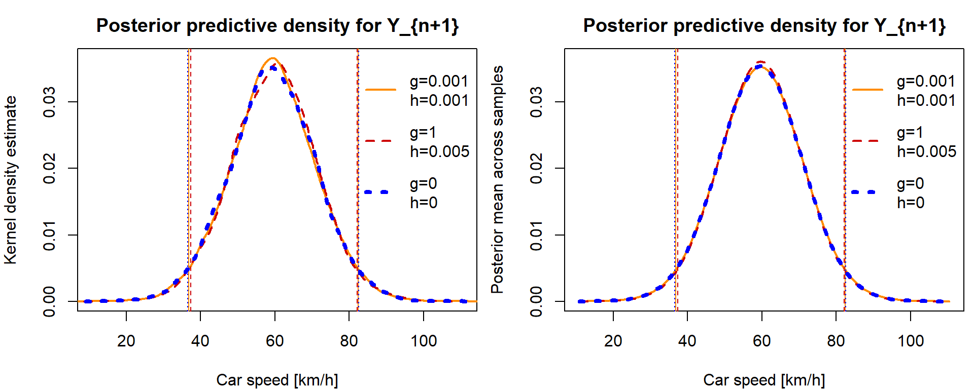

Task 11 - Posterior probability

Extend a bit more the function which generates from the posterior distribution \(p(\mu,\,\tau\,|\,\mathbb{Y})\) and calculate the Monte Carlo estimate of a probability that another car exceeds the allowed speed by more than 30 km/h (and the driver loses their driving license for certain period of time).

Note an analogue of the relationship from Task 9: \[\begin{equation*} \mathsf{P}(Y_{n+1} > 80\,|\,\mathbb{Y}) = \int \mathsf{P}(Y_{n+1} > 80\,|\,\mu,\,\tau,\,\mathbb{Y})\, p(\mu,\,\tau\,|\,\mathbb{Y})\, \mathrm{d}(\mu,\,\tau) = \int \mathsf{P}(Y_{n+1} > 80\,|\,\mu,\,\tau)\,p(\mu,\,\tau\,|\,\mathbb{Y})\,\mathrm{d}(\mu,\,\tau). \end{equation*}\]

(prob80 <- lapply(smpls, function(x){mean(x[,"y"] > 80)}))

## [[1]]
## [1] 0.0387
## 
## [[2]]
## [1] 0.0362
## 
## [[3]]
## [1] 0.0385

# could be done as a mean of probabilities from distribution of Y given sampled values of mu and tau
lapply(smpls, function(x){
  mean(pnorm(80, mean = x[,"mu"], sd = 1 / sqrt(x[,"tau"]), lower.tail = FALSE))
})

## [[1]]
## [1] 0.03783848
## 
## [[2]]
## [1] 0.03471622
## 
## [[3]]
## [1] 0.03731408