Bayesian Methods - Ex3a - Linear Mixed-Effects Model
Jan Vávra
This assignment is supposed to be solved via JAGS and
library(runjags). List through the manual
to find what you need.
Data and model description
We will work with the aids data from
library(JM), see help(aids) for more details.
It is of both longitudinal and survival data nature. In this part of the
exercise, we will focus on the longitudinal aspect:
set.seed(123456789)
library(JM)
head(aids[,c("patient", "CD4", "obstime", "drug")], 15)
## patient CD4 obstime drug
## 1 1 10.677078 0 ddC
## 2 1 8.426150 6 ddC
## 3 1 9.433981 12 ddC
## 4 2 6.324555 0 ddI
## 5 2 8.124038 6 ddI
## 6 2 4.582576 12 ddI
## 7 2 5.000000 18 ddI
## 8 3 3.464102 0 ddI
## 9 3 3.605551 2 ddI
## 10 3 6.164414 6 ddI
## 11 4 3.872983 0 ddC
## 12 4 4.582576 2 ddC
## 13 4 2.645751 6 ddC
## 14 4 1.732051 12 ddC
## 15 5 7.280110 0 ddIIt consists of 467 HIV infected patients who were treated with two
antiretroviral drugs (drug).
We will model the evolution of CD4 cell count for each
individual patient.
The time at which the measurement of CD4 was taken is
obstime in months. It is either 0, 2, 6, 12 or 18
(prescribed times of visits). Let us have a look on several random
patients:
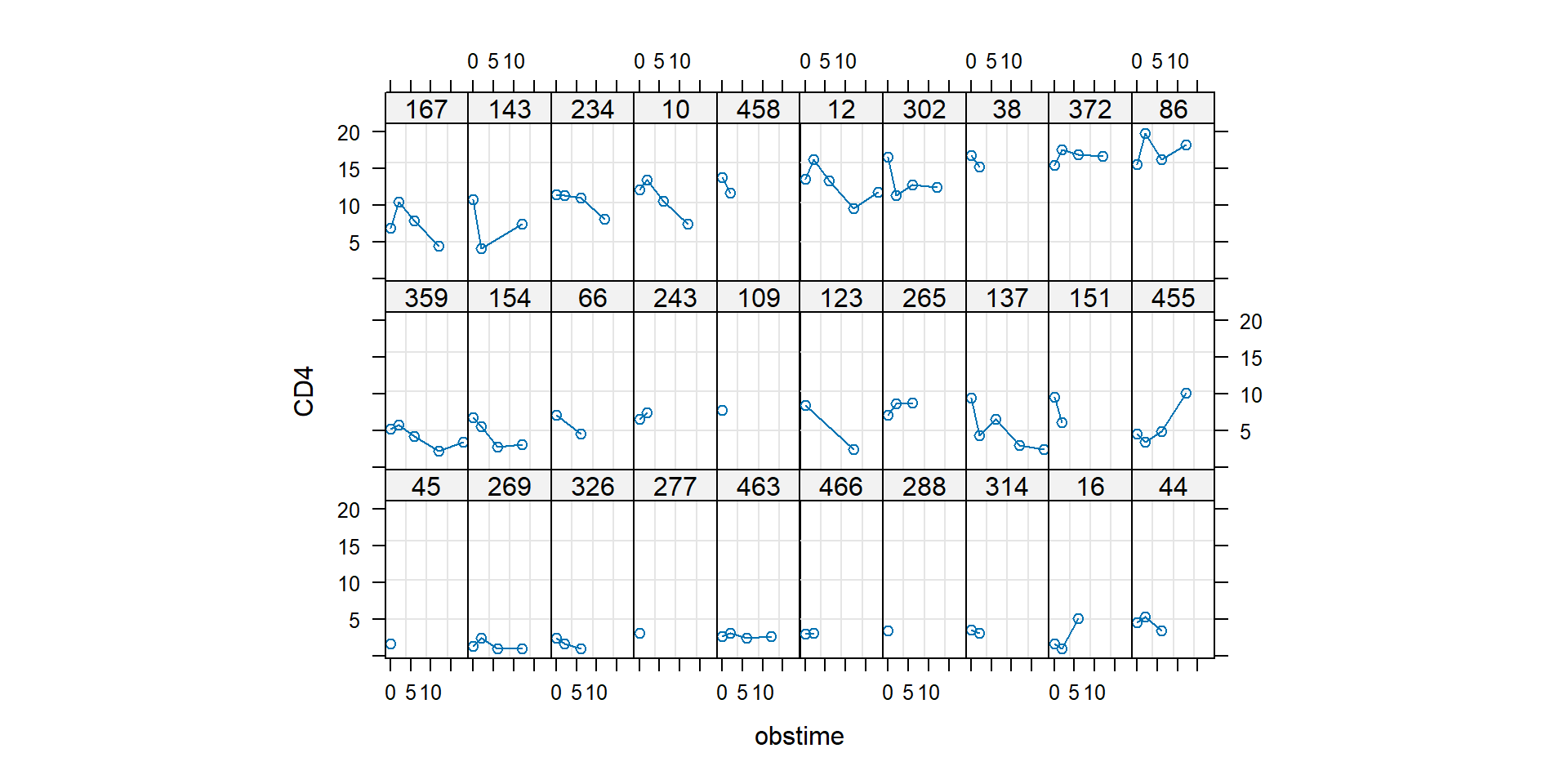 For some people the cell count decreases in time, for some increases. We
will use this observation to construct linear mixed-effects (LME)
model.
For some people the cell count decreases in time, for some increases. We
will use this observation to construct linear mixed-effects (LME)
model.
Task 1 - Frequentistic approach
Fit LME model (e.g. lme from library(nlme))
with random intercept and slope estimated with ML approach:
- \(Y_{ij} = \beta_1 + B_{1i} + (\beta_2 +
B_{2i}) t_{ij} + \beta_3 D_i t_{ij} + \varepsilon_{ij}\), is the
CD4cell count of patient \(i\) at visit \(j\), - \(\varepsilon_{ij} \sim \mathsf{N}(0, \sigma^2)\) is the iid model error,
- \(t_{ij}\) is the time of the observation of patient \(i\) at visit \(j\),
- \(D_i\) is the indicator of
druglevelddI, - \(B_{1i}\) and \(B_{2i}\) are the random intercept and slope for patient \(i\),
- \(\mathbf{B}_i = (B_{1i}, B_{2i})^\top \sim \mathsf{N}_2 (\mathbf{0}, \Sigma)\), where \(\Sigma\) is general positive-definite matrix.
Notice that there is no \(\beta_4 D_i\) within the formula. It would have the interpretation of difference between drug when \(t=0\) (study has not started yet). It is reasonable to assume \(\beta_4 = 0\) and not include it within the model.
Print the summary of the model. Look at the magnitude of the coefficients including standard errors. Use this information to choose non-informative prior in the next Task.
Task 2 - Bayesian approach - JAGS implementation
Consider the same model from Task 1. Reparametrize the variance parameters through precisions instead: \(\tau = \sigma^{-2}\), \(\Omega = \Sigma^{-1}\). Move the parametrization of intercept and slope for patient \(i\) into the prior mean of respective random effects to reduce the autocorrelation: \[ \mathsf{E} \, B_{1i} = \beta_1 \qquad \mathsf{E} \, B_{2i} = \beta_2 + \beta_3 D_i. \] (You can implement other versions with \(\mathsf{E} B_{1i} = 0\) or \(\mathsf{E} B_{2i} = 0\) or \(\mathsf{E} B_{2i} = \beta_2\) to see the difference for yourself.)
Assume the independent block structure of the prior for model
parameters: \[
p(\boldsymbol{\beta}, \tau, \Omega) = \prod\limits_{j=1}^3 p(\beta_j) \,
p(\tau) \, p(\Omega)
\] Choose weakly informative normal prior for \(\beta_j\), gamma prior for \(\tau\) and Wishart distribution
(dwish) for \(\Omega\).
Write down (and print) the model implementation within JAGS.
Task 3 - Running JAGS
Sample two Markov chains using JAGS to approximate the posterior
distribution \(p(\boldsymbol{\beta}, \tau,
\Omega \,|\,\mathsf{data})\). Choose appropriate
burnin and thin by monitoring the trajectories
and autocorrelation.
Task 4 - Monte Carlo estimates
Provide summaries including ET and HPD intervals for primary model parameters. Monitor also standard deviations of random effects and their correlation. Compare them to the outputs in Task 1.