Generalized linear model and nonlinear regression model
Jan Vávra
Exercise 12
Download this R markdown as: R, Rmd.
Outline of this lab session:
- Generalized linear model
- Nonlinear regression model
In normal linear model we assume that the continuous response variable \(Y \in \mathbb{R}\) has given \(p\)-variate covariates \(\mathbf{X} \in \mathbb{R}^p\) the following normal distribution \[ Y | \mathbf{X} \sim \mathsf{N}(\mathbf{X}^\top\boldsymbol{\beta}, \sigma^2), \] where \(\boldsymbol{\beta} \in \mathbb{R}^p\) is the unknown parameter vector and \(\sigma^2 > 0\) is (usually) the unknown variance parameter. The normality assumption is not strictly needed here (exact vs. asymptotic results and inference).
In the general linear regression model, the assumption about the homoscedastic variance is relaxed and the underlying model for the observed data \(\boldsymbol{Y} = (Y_1, \dots, Y_n)^\top\) given the corresponding model matrix \(\mathbb{X} \in \mathbb{R}^{n \times p }\) can be expressed as
\[ \boldsymbol{Y} | \mathbb{X} \sim \mathsf{N}_n(\mathbb{X} \boldsymbol{\beta}, \sigma^2\mathbb{W}^{-1}), \] for some general (positive definite) variance matrix \(\mathbb{W}^{-1}\). Again, the normality assumption in the model above can be omitted.
The concept of a linear model will be further generalized today.
1. Generalized linear model
Firstly, the generalized linear regression model is assumed, where the response variable \(Y\) does not follow the normal distribution any more (either continuous substantially different from normal or even discrete). The conditional expectation of \(Y\) given some vector of the subject specific covariates \(\mathbf{X}\) is modeled using an additional (nonlinear link function) that connects the linear predictor \(\mathbf{X}^\top\boldsymbol{\beta} \in \mathbb{R}\) with the conditional expectation \(\mu_x = \mathsf{E}[Y | \mathbf{X}] \in \mathcal{M} \subseteq \mathbb{R}\).
Typically, the model is assumed in a form \[ \mathsf{E}[Y | \mathbf{X}] = g^{-1}(\mathbf{X}^\top\boldsymbol{\beta}), \] where \(g(\cdot)\) is the so-called link function. Its purpose is to map the conditional expectation from \(\mathcal{M}\) onto the whole real line \(\mathbb{R}\) where the predictor lives.
Different models for different distributions of \(Y\) and different link functions \(g(\cdot)\) can be assumed and different statistical properties with different interpretation of the unknown vector of the parameters \(\boldsymbol{\beta} \in \mathbb{R}^p\) follow accordingly.
For illustration purposes we will consider the dataset
mtcars and we will model the consumption of the car given
some additional covariates.
data(mtcars)
mtcars$mpg01 <- as.numeric(mtcars$mpg > 20)
mtcars$fam <- factor(mtcars$am, levels = 0:1, labels = c("Automatic", "Manual"))
summary(mtcars)
## mpg cyl disp hp drat wt
## Min. :10.40 Min. :4.000 Min. : 71.1 Min. : 52.0 Min. :2.760 Min. :1.513
## 1st Qu.:15.43 1st Qu.:4.000 1st Qu.:120.8 1st Qu.: 96.5 1st Qu.:3.080 1st Qu.:2.581
## Median :19.20 Median :6.000 Median :196.3 Median :123.0 Median :3.695 Median :3.325
## Mean :20.09 Mean :6.188 Mean :230.7 Mean :146.7 Mean :3.597 Mean :3.217
## 3rd Qu.:22.80 3rd Qu.:8.000 3rd Qu.:326.0 3rd Qu.:180.0 3rd Qu.:3.920 3rd Qu.:3.610
## Max. :33.90 Max. :8.000 Max. :472.0 Max. :335.0 Max. :4.930 Max. :5.424
## qsec vs am gear carb mpg01
## Min. :14.50 Min. :0.0000 Min. :0.0000 Min. :3.000 Min. :1.000 Min. :0.0000
## 1st Qu.:16.89 1st Qu.:0.0000 1st Qu.:0.0000 1st Qu.:3.000 1st Qu.:2.000 1st Qu.:0.0000
## Median :17.71 Median :0.0000 Median :0.0000 Median :4.000 Median :2.000 Median :0.0000
## Mean :17.85 Mean :0.4375 Mean :0.4062 Mean :3.688 Mean :2.812 Mean :0.4375
## 3rd Qu.:18.90 3rd Qu.:1.0000 3rd Qu.:1.0000 3rd Qu.:4.000 3rd Qu.:4.000 3rd Qu.:1.0000
## Max. :22.90 Max. :1.0000 Max. :1.0000 Max. :5.000 Max. :8.000 Max. :1.0000
## fam
## Automatic:19
## Manual :13
##
##
##
## In the following we will fit different models and we will compare the outputs. We start with ordinary linear model:
m <- list()
m[["lm"]] <- lm(mpg ~ disp + fam, data = mtcars)
summary(m[["lm"]])
##
## Call:
## lm(formula = mpg ~ disp + fam, data = mtcars)
##
## Residuals:
## Min 1Q Median 3Q Max
## -4.6382 -2.4751 -0.5631 2.2333 6.8386
##
## Coefficients:
## Estimate Std. Error t value Pr(>|t|)
## (Intercept) 27.848081 1.834071 15.184 2.45e-15 ***
## disp -0.036851 0.005782 -6.373 5.75e-07 ***
## famManual 1.833458 1.436100 1.277 0.212
## ---
## Signif. codes: 0 '***' 0.001 '**' 0.01 '*' 0.05 '.' 0.1 ' ' 1
##
## Residual standard error: 3.218 on 29 degrees of freedom
## Multiple R-squared: 0.7333, Adjusted R-squared: 0.7149
## F-statistic: 39.87 on 2 and 29 DF, p-value: 4.749e-09Generalized linear model with the identity link:
m[["glm-N-id"]] <- glm(mpg ~ disp + fam, data = mtcars) # family = gaussian(link = "identity")
summary(m[["glm-N-id"]])
##
## Call:
## glm(formula = mpg ~ disp + fam, data = mtcars)
##
## Coefficients:
## Estimate Std. Error t value Pr(>|t|)
## (Intercept) 27.848081 1.834071 15.184 2.45e-15 ***
## disp -0.036851 0.005782 -6.373 5.75e-07 ***
## famManual 1.833458 1.436100 1.277 0.212
## ---
## Signif. codes: 0 '***' 0.001 '**' 0.01 '*' 0.05 '.' 0.1 ' ' 1
##
## (Dispersion parameter for gaussian family taken to be 10.35453)
##
## Null deviance: 1126.05 on 31 degrees of freedom
## Residual deviance: 300.28 on 29 degrees of freedom
## AIC: 170.46
##
## Number of Fisher Scoring iterations: 2Generalized linear model with the inverse link:
m[["glm-N-inv"]] <- glm(mpg ~ disp + fam, data = mtcars, family = gaussian(link = "inverse"))
summary(m[["glm-N-inv"]])
##
## Call:
## glm(formula = mpg ~ disp + fam, family = gaussian(link = "inverse"),
## data = mtcars)
##
## Coefficients:
## Estimate Std. Error t value Pr(>|t|)
## (Intercept) 2.740e-02 3.871e-03 7.079 8.69e-08 ***
## disp 1.198e-04 1.638e-05 7.310 4.73e-08 ***
## famManual -2.306e-03 2.761e-03 -0.835 0.41
## ---
## Signif. codes: 0 '***' 0.001 '**' 0.01 '*' 0.05 '.' 0.1 ' ' 1
##
## (Dispersion parameter for gaussian family taken to be 7.053581)
##
## Null deviance: 1126.05 on 31 degrees of freedom
## Residual deviance: 204.55 on 29 degrees of freedom
## AIC: 158.17
##
## Number of Fisher Scoring iterations: 6Generalized linear model for the binary response with logit link - logistic regression:
m[["glm-bin-logit"]] <- glm(mpg01 ~ disp + fam, data = mtcars, family = binomial) # link = "logit"
summary(m[["glm-bin-logit"]])
##
## Call:
## glm(formula = mpg01 ~ disp + fam, family = binomial, data = mtcars)
##
## Coefficients:
## Estimate Std. Error z value Pr(>|z|)
## (Intercept) 5.1245 2.3231 2.206 0.0274 *
## disp -0.0287 0.0116 -2.473 0.0134 *
## famManual 0.6140 1.4011 0.438 0.6612
## ---
## Signif. codes: 0 '***' 0.001 '**' 0.01 '*' 0.05 '.' 0.1 ' ' 1
##
## (Dispersion parameter for binomial family taken to be 1)
##
## Null deviance: 43.860 on 31 degrees of freedom
## Residual deviance: 16.381 on 29 degrees of freedom
## AIC: 22.381
##
## Number of Fisher Scoring iterations: 7Generalized linear model for the binary response with probit link - probit regression:
m[["glm-bin-probit"]] <- glm(mpg01 ~ disp + fam, data = mtcars, family = binomial(link = "probit"))
summary(m[["glm-bin-probit"]])
##
## Call:
## glm(formula = mpg01 ~ disp + fam, family = binomial(link = "probit"),
## data = mtcars)
##
## Coefficients:
## Estimate Std. Error z value Pr(>|z|)
## (Intercept) 3.033994 1.253200 2.421 0.01548 *
## disp -0.016560 0.005878 -2.817 0.00484 **
## famManual 0.302270 0.783313 0.386 0.69958
## ---
## Signif. codes: 0 '***' 0.001 '**' 0.01 '*' 0.05 '.' 0.1 ' ' 1
##
## (Dispersion parameter for binomial family taken to be 1)
##
## Null deviance: 43.860 on 31 degrees of freedom
## Residual deviance: 16.155 on 29 degrees of freedom
## AIC: 22.155
##
## Number of Fisher Scoring iterations: 8Predictions based on glm class of models depend on
family, link and purpose. We start with
family = gaussian(...):
newdata <- list()
for(f in levels(mtcars$fam)){
  newdata[[f]] <- data.frame(disp = seq(min(mtcars$disp), max(mtcars$disp), length.out = 101),
                             fam = f)
}
BGf <- c("yellowgreen", "plum")
COLf <- c("forestgreen", "magenta")
names(COLf) <- names(BGf) <- levels(mtcars$fam)

par(mfrow = c(1,2), mar = c(4,4,2.5,0.5))
for(f in levels(mtcars$fam)){
  plot(mpg ~ disp, data = mtcars,
       xlab = expression(Displacement~"["~inch^3~"]"), ylab = "Miles per gallon",
       main = paste0("Transmission = ", f),
       pch = 21, col = ifelse(mtcars$fam==f, COLf[f], "black"), bg = ifelse(mtcars$fam==f, BGf[f], "grey"))
  abline(h = 20, col = "slategrey", lty = 2)
  lines(x = newdata[[f]]$disp, y = predict(m[["glm-N-id"]], newdata[[f]], type = "response"),
        col = "blue", lty = 1, lwd = 2)
  lines(x = newdata[[f]]$disp, y = predict(m[["glm-N-inv"]], newdata[[f]], type = "response"),
        col = "red", lty = 1, lwd = 2)
  legend("topright", c("link = identity", "link = inverse"), bty = "n",
         title = "family = gaussian", col = c("blue", "red"), lwd = 2)
  legend("bottomleft", levels(mtcars$fam), bty = "n",
         pt.bg = ifelse(levels(mtcars$fam)==f, BGf[f], "grey"),
         col = ifelse(levels(mtcars$fam)==f, COLf[f], "black"),
         pch = 21, pt.cex = 1.5)
}
Linear predictor for binary mpg01 = mpg > 20 -
predict type="link":
par(mfrow = c(1,2), mar = c(4,4,2.5,0.5))
for(f in levels(mtcars$fam)){
  plogit <- predict(m[["glm-bin-logit"]], newdata[[f]], type = "link")
  pprobit <- predict(m[["glm-bin-probit"]], newdata[[f]], type = "link")
  plot(plogit ~ newdata[[f]]$disp, type = "l",
       xlab = expression(Displacement~"["~inch^3~"]"), ylab = "Linear predictor",
       ylim = range(plogit, pprobit),
       main = paste0("Transmission = ", f),
       col = "blue", lty = 1, lwd = 2)
  lines(pprobit ~ newdata[[f]]$disp, col = "red", lty = 1, lwd = 2)
  legend("topright", c("link = logit", "link = probit"), bty = "n",
         title = "family = binomial", col = c("blue", "red"), lwd = 2)
}
Estimated probability of mpg01 = mpg > 20 - predict
type="response":
par(mfrow = c(1,2), mar = c(4,4,2.5,0.5))
for(f in levels(mtcars$fam)){
  plogit <- predict(m[["glm-bin-logit"]], newdata[[f]], type = "response")
  pprobit <- predict(m[["glm-bin-probit"]], newdata[[f]], type = "response")
  plot(plogit ~ newdata[[f]]$disp, type = "l",
       xlab = expression(Displacement~"["~inch^3~"]"), ylab = "Probability(MPG > 20)",
       ylim = c(0,1),
       main = paste0("Transmission = ", f),
       col = "blue", lty = 1, lwd = 2)
  lines(pprobit ~ newdata[[f]]$disp, col = "red", lty = 1, lwd = 2)
  legend("topright", c("link = logit", "link = probit"), bty = "n",
         title = "family = binomial", col = c("blue", "red"), lwd = 2)
}
Individual work
- Discuss and compare the models above. Which ones can be compared directly? Can you explain the differences that you observe?
- What is the corresponding interpretation of all the parameters being estimated in the models above?
- What are the conclusions between the model with the continuous
response
mpgand its dichotomous versionmpg01? - Which of the estimated parameters in the three models above can you reconstruct manually?
2. Nonlinear regression model
The second generalization of the linear regression model involves the change of the linear predictor \(\boldsymbol{X}^\top\boldsymbol{\beta}\) into a nonlinear predictor \(f(\boldsymbol{X}, \boldsymbol{\beta})\), for some well-specified regression function \(f: \mathbb{R}^{p \times q} \to \mathcal{M}\) (with an analytic formula that depends on the parameter vector \(\boldsymbol{\beta} \in \mathbb{R}^q\)).
Nonlinear regression models in R can be fitted by using the command
nls() (nonlinear least squares) – see the corresponding
help session for more details (?nls).
Compare the following two models:
- ordinary linear model:
m[["lm"]] <- lm(mpg ~ disp + am, data = mtcars)
summary(m[["lm"]])
##
## Call:
## lm(formula = mpg ~ disp + am, data = mtcars)
##
## Residuals:
## Min 1Q Median 3Q Max
## -4.6382 -2.4751 -0.5631 2.2333 6.8386
##
## Coefficients:
## Estimate Std. Error t value Pr(>|t|)
## (Intercept) 27.848081 1.834071 15.184 2.45e-15 ***
## disp -0.036851 0.005782 -6.373 5.75e-07 ***
## am 1.833458 1.436100 1.277 0.212
## ---
## Signif. codes: 0 '***' 0.001 '**' 0.01 '*' 0.05 '.' 0.1 ' ' 1
##
## Residual standard error: 3.218 on 29 degrees of freedom
## Multiple R-squared: 0.7333, Adjusted R-squared: 0.7149
## F-statistic: 39.87 on 2 and 29 DF, p-value: 4.749e-09- linear model as nonlinear least squares:
start <- list()
start[["nls-as-lm"]] <- c(a = 0, b = 0, c = 0)
m[["nls-as-lm"]] <- nls(mpg ~ a + b * disp + c * am, data = mtcars, start[["nls-as-lm"]])
summary(m[["nls-as-lm"]])
##
## Formula: mpg ~ a + b * disp + c * am
##
## Parameters:
## Estimate Std. Error t value Pr(>|t|)
## a 27.848081 1.834071 15.184 2.45e-15 ***
## b -0.036851 0.005782 -6.373 5.75e-07 ***
## c 1.833458 1.436100 1.277 0.212
## ---
## Signif. codes: 0 '***' 0.001 '**' 0.01 '*' 0.05 '.' 0.1 ' ' 1
##
## Residual standard error: 3.218 on 29 degrees of freedom
##
## Number of iterations to convergence: 1
## Achieved convergence tolerance: 3.547e-09Consider some nonlinear model that will properly fit the scatterplot of the data below:
par(mfrow = c(1,1), mar = c(4,4,0.5,0.5))
plot(mpg ~ disp, data = mtcars,
     xlab = expression(Displacement~"["~inch^3~"]"), ylab = "Miles per Gallon",
     pch = 21, bg = BGf[fam], col = COLf[fam])
legend("topright", legend = levels(mtcars$fam), bty = "n",
       pch = 21, pt.bg = BGf, col = COLf)
For instance, exponential function could be reasonable. Using linear regression we would be able to only fit the following model with fixed choice of constant in exponent:
start[["nls-exp-1"]] <- c(a = 0, b = 0)
m[["nls-exp-1"]] <- nls(mpg ~ a + b * exp(-disp/500), data = mtcars, start[["nls-exp-1"]])
summary(m[["nls-exp-1"]])
##
## Formula: mpg ~ a + b * exp(-disp/500)
##
## Parameters:
## Estimate Std. Error t value Pr(>|t|)
## a -2.332 2.347 -0.994 0.328
## b 34.566 3.525 9.807 7.19e-11 ***
## ---
## Signif. codes: 0 '***' 0.001 '**' 0.01 '*' 0.05 '.' 0.1 ' ' 1
##
## Residual standard error: 2.987 on 30 degrees of freedom
##
## Number of iterations to convergence: 1
## Achieved convergence tolerance: 1.229e-09To find reasonable constant in exponent we can make it another model parameter:
# A successful run requires proper setting of initial values
a.0 <- min(mtcars$mpg) * 0.5
auxlm <- lm(log(mpg - a.0) ~ disp, data=mtcars)
start[["nls-exp-2"]] <- c(a.0, exp(coef(auxlm)[1]), coef(auxlm)[2])
names(start[["nls-exp-2"]]) <- letters[1:3]
# end of finding reasonable starting values
m[["nls-exp-2"]] <- nls(mpg ~ a + b * exp(c * disp), data = mtcars, start[["nls-exp-2"]])
summary(m[["nls-exp-2"]])
##
## Formula: mpg ~ a + b * exp(c * disp)
##
## Parameters:
## Estimate Std. Error t value Pr(>|t|)
## a 14.50544 0.94383 15.369 1.79e-15 ***
## b 40.26532 7.94320 5.069 2.09e-05 ***
## c -0.01188 0.00247 -4.810 4.30e-05 ***
## ---
## Signif. codes: 0 '***' 0.001 '**' 0.01 '*' 0.05 '.' 0.1 ' ' 1
##
## Residual standard error: 2.437 on 29 degrees of freedom
##
## Number of iterations to convergence: 11
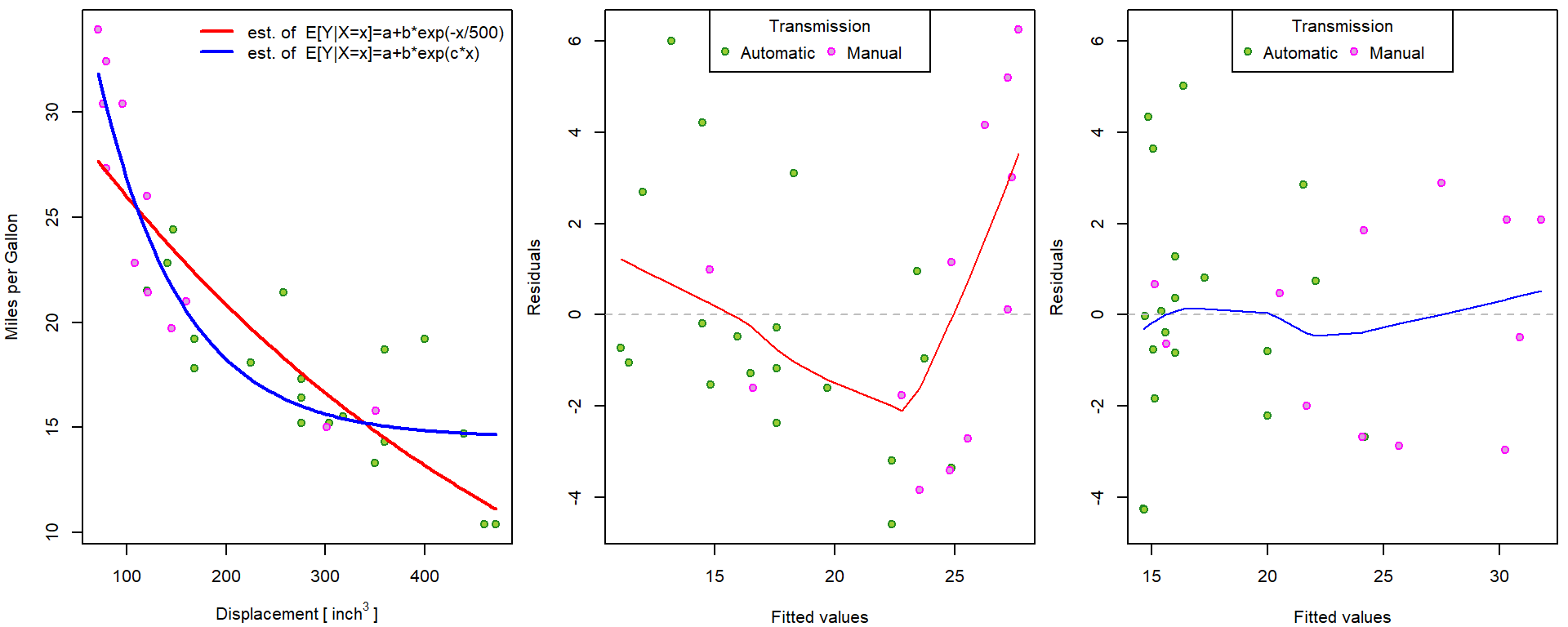
## Achieved convergence tolerance: 5.721e-06The model can be fitted into the data as follows:
pred <- list()
xgrid <- seq(min(mtcars$disp), max(mtcars$disp), length = 101)
pred_manual <- coef(m[["nls-exp-1"]])[1] + coef(m[["nls-exp-1"]])[2] * exp(- xgrid/500)
pred[["nls-exp-1"]] <- predict(m[["nls-exp-1"]], newdata = data.frame(disp = xgrid))
all.equal(pred[["nls-exp-1"]], pred_manual)
## [1] TRUEpred[["nls-exp-2"]] <- predict(m[["nls-exp-2"]], newdata = data.frame(disp = xgrid))
COLm <- c("red", "blue")
names(COLm) <- c("nls-exp-1", "nls-exp-2")
par(mfrow = c(1,3), mar = c(4,4,0.5,0.5))
plot(mpg ~ disp, data = mtcars,
xlab = expression(Displacement~"["~inch^3~"]"), ylab = "Miles per Gallon",
pch = 21, bg = BGf[fam], col = COLf[fam])
for(model in c("nls-exp-1", "nls-exp-2")){
lines(pred[[model]] ~ xgrid, col = COLm[model], lwd = 2)
}
legend("topright", bty = "n",
legend = c("est. of E[Y|X=x]=a+b*exp(-x/500)",
"est. of E[Y|X=x]=a+b*exp(c*x)"),
col = COLm, lwd = 2, lty = 1)
# residuals vs fitted - own implementation
res_fit <- function(m, YLIM = range(residuals(m))){
plot(residuals(m) ~ fitted(m),
xlab = "Fitted values", ylab = "Residuals",
ylim = YLIM, pch = 21, bg = BGf[mtcars$fam], col = COLf[mtcars$fam])
abline(h=0, col = "grey", lty = 2)
lines(lowess(residuals(m) ~ fitted(m)), col = COLm[model])
legend("top", legend = levels(mtcars$fam), ncol = 2,
title = "Transmission", pch = 21, pt.bg = BGf, col = COLf)
}
YLIM <- range(residuals(m[["nls-exp-1"]]), residuals(m[["nls-exp-2"]]))
for(model in c("nls-exp-1", "nls-exp-2")){
res_fit(m[[model]], YLIM = YLIM)
}
How to include different exponential functions for different transmission?
model <- "nls-exp-by-am"
start[[model]] <- c(coef(m[["nls-exp-2"]]), rep(0, 3))
names(start[[model]]) <- letters[1:6]
m[[model]] <- nls(mpg ~ (a+d*am) + (b+e*am) * exp((c+f*am)*disp), data = mtcars, start[[model]])
summary(m[[model]])
##
## Formula: mpg ~ (a + d * am) + (b + e * am) * exp((c + f * am) * disp)
##
## Parameters:
## Estimate Std. Error t value Pr(>|t|)
## a -2.523e+01 2.318e+02 -0.109 0.9141
## b 5.110e+01 2.278e+02 0.224 0.8243
## c -6.524e-04 3.575e-03 -0.183 0.8566
## d 4.037e+01 2.318e+02 0.174 0.8631
## e -2.488e+00 2.282e+02 -0.011 0.9914
## f -1.384e-02 5.699e-03 -2.428 0.0224 *
## ---
## Signif. codes: 0 '***' 0.001 '**' 0.01 '*' 0.05 '.' 0.1 ' ' 1
##
## Residual standard error: 2.366 on 26 degrees of freedom
##
## Number of iterations to convergence: 17
## Achieved convergence tolerance: 6.558e-06predy_aut <- predict(m[[model]], newdata = data.frame(disp = xgrid, am = 0))
predy_man <- predict(m[[model]], newdata = data.frame(disp = xgrid, am = 1))
par(mfrow = c(1,2), mar = c(4,4,0.5,0.5))
plot(mpg ~ disp, data = mtcars,
xlab = expression(Displacement~"["~inch^3~"]"), ylab = "Miles per Gallon",
pch = 21, bg = BGf[fam], col = COLf[fam])
lines(predy_aut ~ xgrid, col = COLf["Automatic"], lwd = 2)
lines(predy_man ~ xgrid, col = COLf["Manual"], lwd = 2)
legend("topright", legend = levels(mtcars$fam), bty = "n",
lty = 1, lwd = 2, col = COLf)
COLm[model] <- "red"
res_fit(m[[model]])
Individual work
- Compare the model above with a standard linear regression model.
- Design a formula that would have linear trend for Automatic and exponential trend for Manual.
- Consider also models where the response
mpgwould be transformed by logarithm.