Review of statistical methods
Jan Vávra
Exercise 1
Download this R markdown as: R, Rmd.
Loading the data and libraries
If you use your personal computer an additional package
mffSM is needed. The package is not available from CRAN but
can be downloaded from this website. Download the package and use the following
command for the installation:
install.packages("mffSM_1.1.zip", repos = NULL)
# or without necessity to download first
install.packages("https://www2.karlin.mff.cuni.cz/~komarek/vyuka/2021_22/nmsa407/R/mffSM_1.2.tar.gz", repos = NULL)
Libraries can be accessed the following way. When in doubt, use
help() or ? to show the documentation:
library("mffSM")
library("colorspace")
help(package="mffSM")
This lab session we will work with the data set on car vehicles that were on the market in the U.S. in 2004:
data(Cars2004nh, package = "mffSM")Quick overview and summary of the data:
dim(Cars2004nh)## [1] 425 20str(Cars2004nh)## 'data.frame': 425 obs. of 20 variables:
## $ vname : chr "Chevrolet.Aveo.4dr" "Chevrolet.Aveo.LS.4dr.hatch" "Chevrolet.Cavalier.2dr" "Chevrolet.Cavalier.4dr" ...
## $ type : int 1 1 1 1 1 1 1 1 1 1 ...
## $ drive : int 1 1 1 1 1 1 1 1 1 1 ...
## $ price.retail: int 11690 12585 14610 14810 16385 13670 15040 13270 13730 15460 ...
## $ price.dealer: int 10965 11802 13697 13884 15357 12849 14086 12482 12906 14496 ...
## $ price : num 11328 12194 14154 14347 15871 ...
## $ cons.city : num 8.4 8.4 9 9 9 8.1 8.1 9 8.7 9 ...
## $ cons.highway: num 6.9 6.9 6.4 6.4 6.4 6.5 6.5 7.1 6.5 7.1 ...
## $ consumption : num 7.65 7.65 7.7 7.7 7.7 7.3 7.3 8.05 7.6 8.05 ...
## $ engine.size : num 1.6 1.6 2.2 2.2 2.2 2 2 2 2 2 ...
## $ ncylinder : int 4 4 4 4 4 4 4 4 4 4 ...
## $ horsepower : int 103 103 140 140 140 132 132 130 110 130 ...
## $ weight : int 1075 1065 1187 1214 1187 1171 1191 1185 1182 1182 ...
## $ iweight : num 0.00093 0.000939 0.000842 0.000824 0.000842 ...
## $ lweight : num 6.98 6.97 7.08 7.1 7.08 ...
## $ wheel.base : int 249 249 264 264 264 267 267 262 262 262 ...
## $ length : int 424 389 465 465 465 442 442 427 427 427 ...
## $ width : int 168 168 175 173 175 170 170 170 170 170 ...
## $ ftype : Factor w/ 6 levels "personal","wagon",..: 1 1 1 1 1 1 1 1 1 1 ...
## $ fdrive : Factor w/ 3 levels "front","rear",..: 1 1 1 1 1 1 1 1 1 1 ...head(Cars2004nh)## vname type drive price.retail price.dealer price cons.city cons.highway consumption
## 1 Chevrolet.Aveo.4dr 1 1 11690 10965 11327.5 8.4 6.9 7.65
## 2 Chevrolet.Aveo.LS.4dr.hatch 1 1 12585 11802 12193.5 8.4 6.9 7.65
## 3 Chevrolet.Cavalier.2dr 1 1 14610 13697 14153.5 9.0 6.4 7.70
## 4 Chevrolet.Cavalier.4dr 1 1 14810 13884 14347.0 9.0 6.4 7.70
## 5 Chevrolet.Cavalier.LS.2dr 1 1 16385 15357 15871.0 9.0 6.4 7.70
## 6 Dodge.Neon.SE.4dr 1 1 13670 12849 13259.5 8.1 6.5 7.30
## engine.size ncylinder horsepower weight iweight lweight wheel.base length width ftype fdrive
## 1 1.6 4 103 1075 0.0009302326 6.980076 249 424 168 personal front
## 2 1.6 4 103 1065 0.0009389671 6.970730 249 389 168 personal front
## 3 2.2 4 140 1187 0.0008424600 7.079184 264 465 175 personal front
## 4 2.2 4 140 1214 0.0008237232 7.101676 264 465 173 personal front
## 5 2.2 4 140 1187 0.0008424600 7.079184 264 465 175 personal front
## 6 2.0 4 132 1171 0.0008539710 7.065613 267 442 170 personal frontsummary(Cars2004nh)## vname type drive price.retail price.dealer price
## Length:425 Min. :1.000 Min. :1.000 Min. : 10280 Min. : 9875 Min. : 10078
## Class :character 1st Qu.:1.000 1st Qu.:1.000 1st Qu.: 20370 1st Qu.: 18973 1st Qu.: 19601
## Mode :character Median :1.000 Median :1.000 Median : 27905 Median : 25672 Median : 26656
## Mean :2.219 Mean :1.692 Mean : 32866 Mean : 30096 Mean : 31481
## 3rd Qu.:3.000 3rd Qu.:2.000 3rd Qu.: 39235 3rd Qu.: 35777 3rd Qu.: 37514
## Max. :6.000 Max. :3.000 Max. :192465 Max. :173560 Max. :183013
##
## cons.city cons.highway consumption engine.size ncylinder horsepower
## Min. : 6.20 Min. : 5.100 Min. : 5.65 Min. :1.300 Min. :-1.000 Min. :100.0
## 1st Qu.:11.20 1st Qu.: 8.100 1st Qu.: 9.65 1st Qu.:2.400 1st Qu.: 4.000 1st Qu.:165.0
## Median :12.40 Median : 9.000 Median :10.70 Median :3.000 Median : 6.000 Median :210.0
## Mean :12.36 Mean : 9.142 Mean :10.75 Mean :3.208 Mean : 5.791 Mean :216.8
## 3rd Qu.:13.80 3rd Qu.: 9.800 3rd Qu.:11.65 3rd Qu.:3.900 3rd Qu.: 6.000 3rd Qu.:255.0
## Max. :23.50 Max. :19.600 Max. :21.55 Max. :8.300 Max. :12.000 Max. :500.0
## NA's :14 NA's :14 NA's :14
## weight iweight lweight wheel.base length width
## Min. : 923 Min. :0.0003066 Min. :6.828 Min. :226.0 Min. :363.0 Min. :163.0
## 1st Qu.:1412 1st Qu.:0.0005542 1st Qu.:7.253 1st Qu.:262.0 1st Qu.:450.0 1st Qu.:175.0
## Median :1577 Median :0.0006341 Median :7.363 Median :272.0 Median :472.0 Median :180.0
## Mean :1626 Mean :0.0006412 Mean :7.373 Mean :274.9 Mean :470.6 Mean :181.1
## 3rd Qu.:1804 3rd Qu.:0.0007082 3rd Qu.:7.498 3rd Qu.:284.0 3rd Qu.:490.0 3rd Qu.:185.0
## Max. :3261 Max. :0.0010834 Max. :8.090 Max. :366.0 Max. :577.0 Max. :206.0
## NA's :2 NA's :2 NA's :2 NA's :2 NA's :26 NA's :28
## ftype fdrive
## personal:242 front:223
## wagon : 30 rear :110
## SUV : 60 4x4 : 92
## pickup : 24
## sport : 49
## minivan : 20
## Data subsampling and preprocessing
Exclude cars where the consumption is missing:
Cars2004nh <- Cars2004nh[!is.na(Cars2004nh$consumption),] Create a working subsample:
set.seed(123456789)
idx <- c(sample((1:nrow(Cars2004nh))[Cars2004nh$ftype=="personal"], size=100),
         sample((1:nrow(Cars2004nh))[Cars2004nh$ftype!="personal"], size=120))
Cars2004nh <- Cars2004nh[idx,]
Next, we derive some additional variables. First, binary factor
fdrive2, which distinguishes whether the drive is
front or other (rear or
4x4):
Cars2004nh <- transform(Cars2004nh,
                        fdrive2 = factor(1*(fdrive == "front") + 2*(fdrive != "front"),
                                         labels = c("front", "other")))
with(Cars2004nh, table(fdrive, fdrive2))
## fdrive2
## fdrive front other
## front 102 0
## rear 0 61
## 4x4 0 57Alternatively, it could be done by changing labels:
Cars2004nh <- transform(Cars2004nh,
                        fdrive2 = factor(fdrive,
                                         levels = c("front", "rear", "4x4"),
                                         labels = c("front", "other", "other")))
Next, we derive binary indicator cons10 of having a
consumption <= 10 l/100 km and then create a factor with
No (0) and Yes (1) labels:
Cars2004nh <- transform(Cars2004nh,
                        cons10  = 1 * (consumption <= 10), # 0 or 1
                        fcons10 = factor(1 * (consumption <= 10),
                                         labels = c("No", "Yes")))

summary(Cars2004nh)
## vname type drive price.retail price.dealer price
## Length:220 Min. :1.000 Min. :1.000 Min. : 10760 Min. : 10144 Min. : 10452
## Class :character 1st Qu.:1.000 1st Qu.:1.000 1st Qu.: 20969 1st Qu.: 19468 1st Qu.: 20313
## Mode :character Median :2.000 Median :2.000 Median : 26991 Median : 24876 Median : 25900
## Mean :2.527 Mean :1.795 Mean : 32516 Mean : 29759 Mean : 31138
## 3rd Qu.:4.000 3rd Qu.:3.000 3rd Qu.: 38931 3rd Qu.: 35494 3rd Qu.: 37500
## Max. :6.000 Max. :3.000 Max. :128420 Max. :119600 Max. :124010
##
## cons.city cons.highway consumption engine.size ncylinder horsepower
## Min. : 6.50 Min. : 5.30 Min. : 5.900 Min. :1.300 Min. :-1.000 Min. :103.0
## 1st Qu.:11.20 1st Qu.: 8.10 1st Qu.: 9.688 1st Qu.:2.400 1st Qu.: 4.000 1st Qu.:169.5
## Median :12.40 Median : 9.00 Median :10.700 Median :3.000 Median : 6.000 Median :210.0
## Mean :12.59 Mean : 9.37 Mean :10.978 Mean :3.230 Mean : 5.814 Mean :214.4
## 3rd Qu.:13.80 3rd Qu.:10.20 3rd Qu.:12.037 3rd Qu.:3.925 3rd Qu.: 6.000 3rd Qu.:242.8
## Max. :23.50 Max. :19.60 Max. :21.550 Max. :6.000 Max. :12.000 Max. :493.0
##
## weight iweight lweight wheel.base length width
## Min. : 923 Min. :0.0003445 Min. :6.828 Min. :226.0 Min. :381.0 Min. :163
## 1st Qu.:1440 1st Qu.:0.0005442 1st Qu.:7.272 1st Qu.:262.0 1st Qu.:450.0 1st Qu.:175
## Median :1584 Median :0.0006315 Median :7.367 Median :272.0 Median :470.0 Median :180
## Mean :1646 Mean :0.0006347 Mean :7.384 Mean :275.6 Mean :468.3 Mean :181
## 3rd Qu.:1838 3rd Qu.:0.0006944 3rd Qu.:7.516 3rd Qu.:284.8 3rd Qu.:488.0 3rd Qu.:185
## Max. :2903 Max. :0.0010834 Max. :7.973 Max. :366.0 Max. :556.0 Max. :206
## NA's :2 NA's :2 NA's :2 NA's :18 NA's :19
## ftype fdrive fdrive2 cons10 fcons10
## personal:100 front:102 front:102 Min. :0.0000 No :144
## wagon : 19 rear : 61 other:118 1st Qu.:0.0000 Yes: 76
## SUV : 41 4x4 : 57 Median :0.0000
## pickup : 18 Mean :0.3455
## sport : 29 3rd Qu.:1.0000
## minivan : 13 Max. :1.0000
## Two sample problem
In this section, we review the methods for two-sample problems, i.e. exploring the relationship between continuous variable and binary variable. In particular, we are going to explore the following question:
Does the consumption depend on the drive while distinguishing only two categories: front and other?
Exploration
We start with an exploration phase. The most straightforward
visualization tool for this problem is boxplot, the default
plot for numeric ~ factor:
plot(consumption ~ fdrive2, data = Cars2004nh)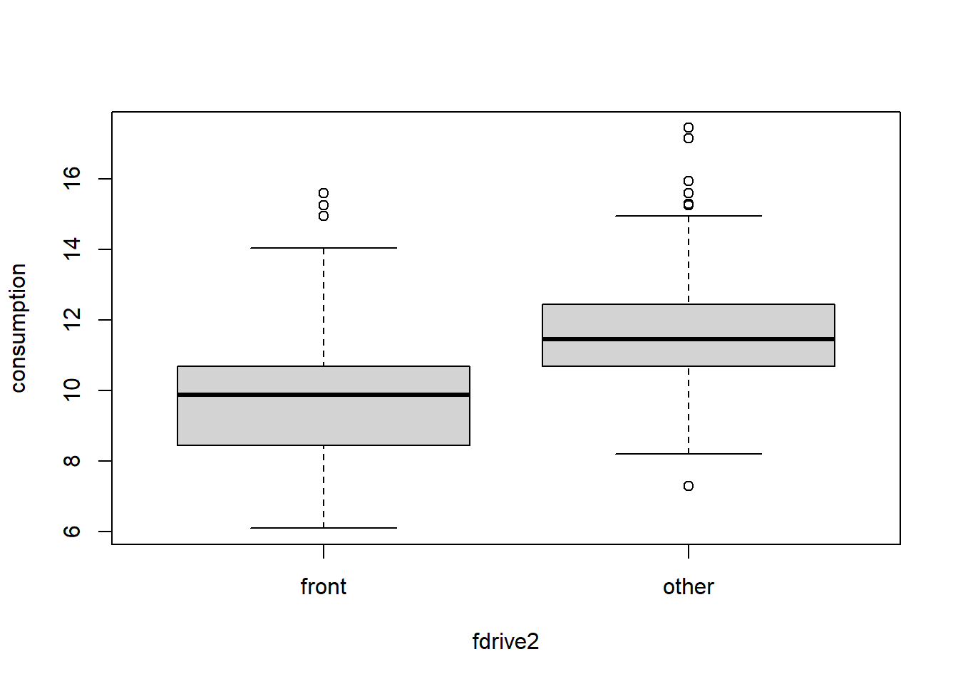
With some effort you can make this plot more compelling:
COL <- c("yellowgreen", "goldenrod")
names(COL) <- levels(Cars2004nh$fdrive2)

par(mfrow = c(1,1), mar = c(4,4,1.5,0.5))
plot(consumption ~ fdrive2, data = Cars2004nh, col = COL,
     xlab = "Drive of the vehicle", ylab = "Consumption [l/100 km]",
     main = "Consumption vs. Front drive",
     cex.main = 1.0,
     xaxt = "n")
axis(1, at = 1:nlevels(Cars2004nh$fdrive2), labels = c("Front drive", "Other"))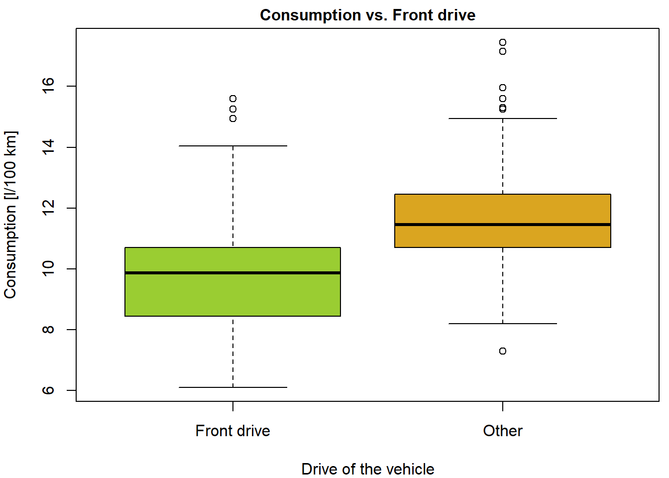
Boxplots of consumption for two categories of drive.
Think about other ways of displaying the two different distributions. Here are the sample characteristics:
with(Cars2004nh, tapply(consumption, fdrive2, summary))## $front
## Min. 1st Qu. Median Mean 3rd Qu. Max.
## 5.900 8.625 9.800 9.866 10.700 15.250
##
## $other
## Min. 1st Qu. Median Mean 3rd Qu. Max.
## 8.95 10.40 11.45 11.94 13.40 21.55with(Cars2004nh, tapply(consumption, fdrive2, sd, na.rm = TRUE))## front other
## 1.868554 2.071336X = subset(Cars2004nh, fdrive2 == "front")$consumption
Y = subset(Cars2004nh, fdrive2 == "other")$consumptionFormal statistical test(s)
For each test refresh the following:
- What is the underlying model in each test?
- What are the assumptions?
Standard two-sample t-test (assuming equal variances and normality)
t.test(consumption ~ fdrive2, data = Cars2004nh, var.equal = TRUE)##
## Two Sample t-test
##
## data: consumption by fdrive2
## t = -7.7434, df = 218, p-value = 3.598e-13
## alternative hypothesis: true difference in means between group front and group other is not equal to 0
## 95 percent confidence interval:
## -2.600394 -1.545219
## sample estimates:
## mean in group front mean in group other
## 9.866176 11.938983mean(X) - mean(Y)## [1] -2.072807Welch two-sample t-test (not assuming equal variances)
t.test(consumption ~ fdrive2, data = Cars2004nh) ##
## Welch Two Sample t-test
##
## data: consumption by fdrive2
## t = -7.8017, df = 217.59, p-value = 2.524e-13
## alternative hypothesis: true difference in means between group front and group other is not equal to 0
## 95 percent confidence interval:
## -2.596457 -1.549156
## sample estimates:
## mean in group front mean in group other
## 9.866176 11.938983Wilcoxon two-sample rank test
wilcox.test(consumption ~ fdrive2, data = Cars2004nh, conf.int = TRUE)##
## Wilcoxon rank sum test with continuity correction
##
## data: consumption by fdrive2
## W = 2638.5, p-value = 6.956e-13
## alternative hypothesis: true location shift is not equal to 0
## 95 percent confidence interval:
## -2.399937 -1.350036
## sample estimates:
## difference in location
## -1.89995median(X) - median(Y)## [1] -1.65XYdiff = outer(X, Y, FUN="-")
median(XYdiff)## [1] -1.9Kolmogorov-Smirnov test
ks.test(consumption ~ fdrive2, data = Cars2004nh)## Warning in ks.test.default(x = DATA[[1L]], y = DATA[[2L]], ...): p-value will be approximate in the presence
## of ties##
## Asymptotic two-sample Kolmogorov-Smirnov test
##
## data: consumption by fdrive2
## D = 0.43553, p-value = 1.938e-09
## alternative hypothesis: two-sidedpar(mfrow = c(1,1), mar = c(4,4,1.5,0.5))
plot(ecdf(X), main="ECDF")
plot(ecdf(Y), col=2, add=TRUE)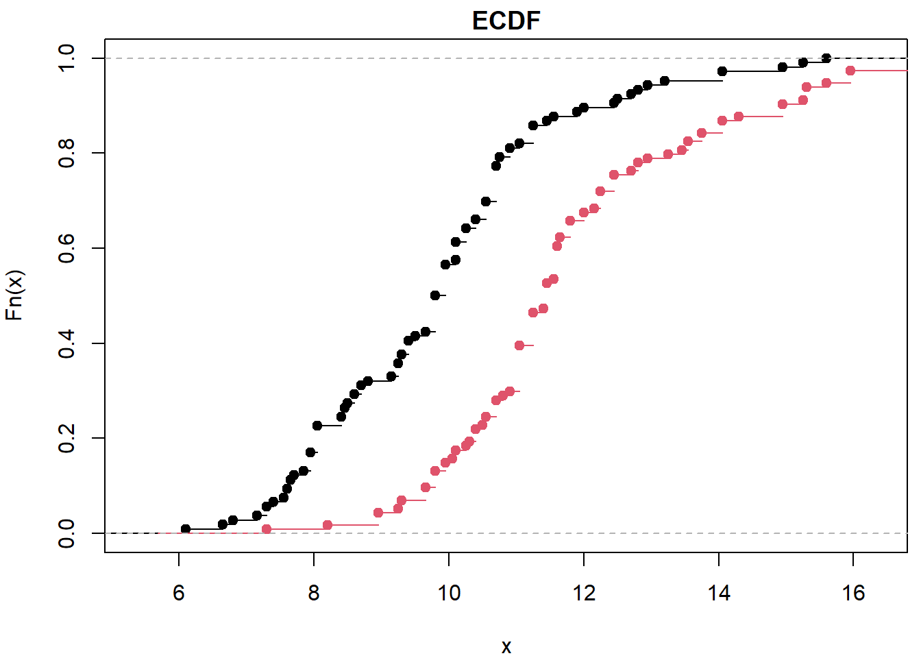
More sample problem
What if there are more than two groups?
Does the consumption depend on the drive (distinguishing front/rear/4x4)?
Exploration
Let’s start with boxplots:
plot(consumption ~ fdrive, data = Cars2004nh)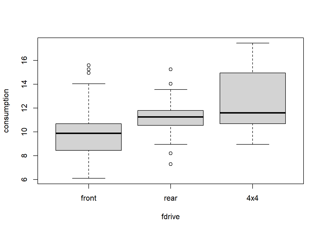
with(Cars2004nh, tapply(consumption, fdrive, summary))## $front
## Min. 1st Qu. Median Mean 3rd Qu. Max.
## 5.900 8.625 9.800 9.866 10.700 15.250
##
## $rear
## Min. 1st Qu. Median Mean 3rd Qu. Max.
## 8.95 10.40 11.05 11.30 11.80 15.25
##
## $`4x4`
## Min. 1st Qu. Median Mean 3rd Qu. Max.
## 9.65 10.55 12.25 12.62 14.05 21.55with(Cars2004nh, tapply(consumption, fdrive, sd, na.rm = TRUE))## front rear 4x4
## 1.868554 1.439618 2.413024Formal statistical test(s)
For each test refresh the following:
- What is the underlying model in each test?
- What are the assumptions?
Standard ANOVA
summary(aov(consumption ~ fdrive, data = Cars2004nh)) ## Df Sum Sq Mean Sq F value Pr(>F)
## fdrive 2 286.6 143.3 38.73 4.15e-15 ***
## Residuals 217 803.1 3.7
## ---
## Signif. codes: 0 '***' 0.001 '**' 0.01 '*' 0.05 '.' 0.1 ' ' 1ANOVA without assuming equal variances
oneway.test(consumption ~ fdrive, data = Cars2004nh) ##
## One-way analysis of means (not assuming equal variances)
##
## data: consumption and fdrive
## F = 32.3, num df = 2.00, denom df = 122.44, p-value = 5.43e-12Kruskal-Wallis Rank Sum Test
kruskal.test(consumption ~ fdrive, data = Cars2004nh) ##
## Kruskal-Wallis rank sum test
##
## data: consumption by fdrive
## Kruskal-Wallis chi-squared = 56.812, df = 2, p-value = 4.607e-13Alternatively: the same test statistics all in the standard ANOVA above
summary(m0 <- lm(consumption ~ fdrive, data=Cars2004nh))##
## Call:
## lm(formula = consumption ~ fdrive, data = Cars2004nh)
##
## Residuals:
## Min 1Q Median 3Q Max
## -3.9662 -1.3540 -0.0945 1.1272 8.9272
##
## Coefficients:
## Estimate Std. Error t value Pr(>|t|)
## (Intercept) 9.8662 0.1905 51.797 < 2e-16 ***
## fdriverear 1.4338 0.3114 4.605 7.03e-06 ***
## fdrive4x4 2.7566 0.3181 8.665 1.05e-15 ***
## ---
## Signif. codes: 0 '***' 0.001 '**' 0.01 '*' 0.05 '.' 0.1 ' ' 1
##
## Residual standard error: 1.924 on 217 degrees of freedom
## Multiple R-squared: 0.263, Adjusted R-squared: 0.2562
## F-statistic: 38.72 on 2 and 217 DF, p-value: 4.152e-15anova(m0)## Analysis of Variance Table
##
## Response: consumption
## Df Sum Sq Mean Sq F value Pr(>F)
## fdrive 2 286.62 143.310 38.725 4.152e-15 ***
## Residuals 217 803.06 3.701
## ---
## Signif. codes: 0 '***' 0.001 '**' 0.01 '*' 0.05 '.' 0.1 ' ' 1oneway.test(consumption ~ fdrive, data = Cars2004nh, var.equal=TRUE) ##
## One-way analysis of means
##
## data: consumption and fdrive
## F = 38.725, num df = 2, denom df = 217, p-value = 4.152e-15Follow these steps to compute the sum of squares and degrees of freedom needed for ANOVA with equal variances:
X = subset(Cars2004nh, fdrive == "front")$consumption
Y = subset(Cars2004nh, fdrive == "rear")$consumption
Z = subset(Cars2004nh, fdrive == "4x4")$consumption
nX = length(X)
nY = length(Y)
nZ = length(Z)
n = nX+nY+nZ
mX = mean(X)
mY = mean(Y)
mZ = mean(Z)
m = mean(c(X,Y,Z))
(SS_between = nX*(m - mX)^2+nY*(m-mY)^2+nZ*(m-mZ)^2)
## [1] 286.6194(SS_error = sum((X - mX)^2)+sum((Y-mY)^2)+sum((Z-mZ)^2))## [1] 803.0612(SS_total = sum((c(X,Y,Z)-m)^2))## [1] 1089.681(Fstat = SS_between/(3-1) / SS_error*(n - 3))## [1] 38.72458Conditional mean / Regression
Now we review the basic methods for describing the relationship between two continuous variables.
- Does the consumption depend on the length?
Exploration
Why are boxplots not reasonable choice? Use scatterplot instead,
default for plot between numeric and
numeric variable.
par(mfrow = c(1,1), mar = c(4,4,0.5,0.5))
plot(consumption ~ length, data = Cars2004nh, col = "red3", bg = "orange", pch = 23)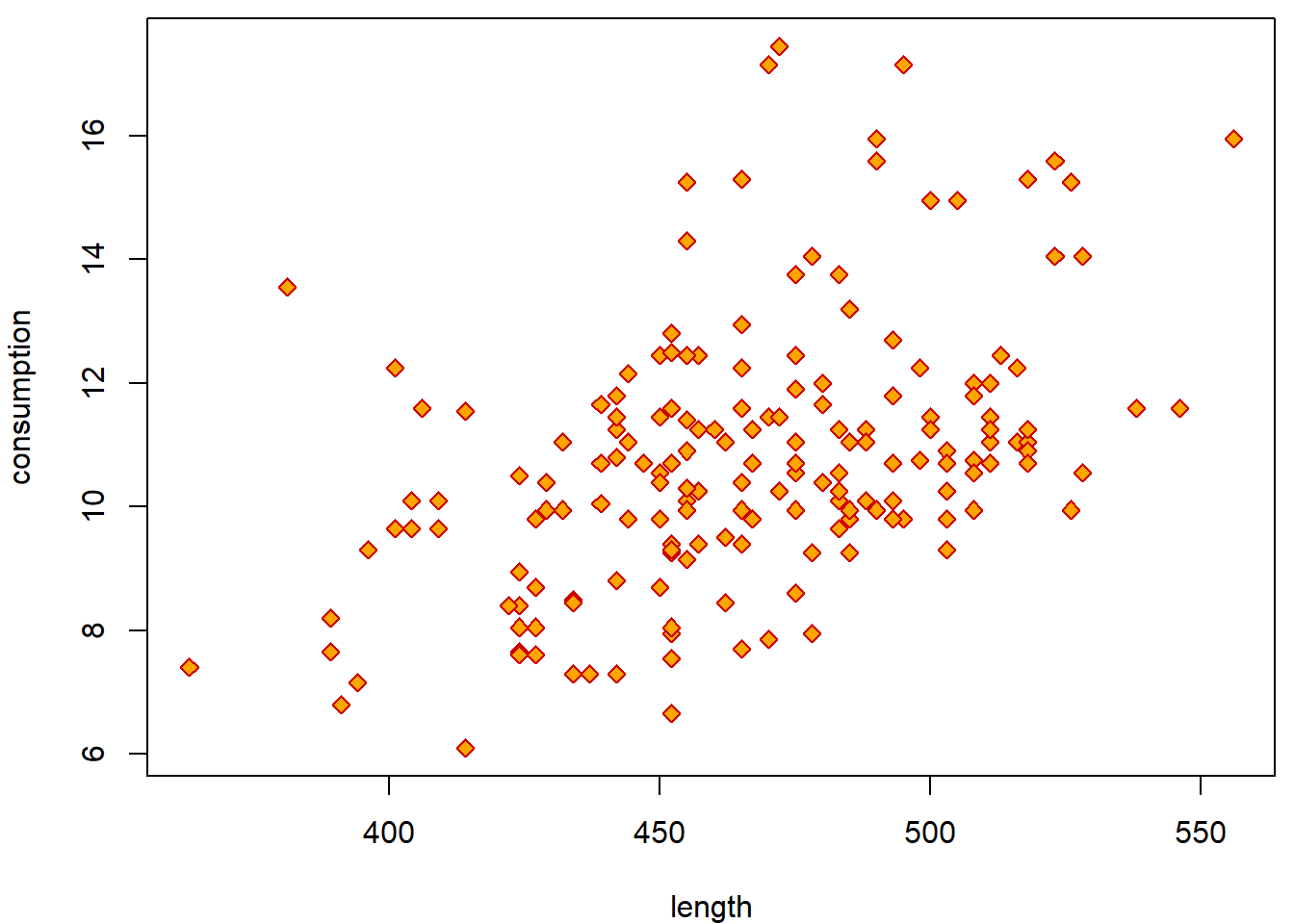
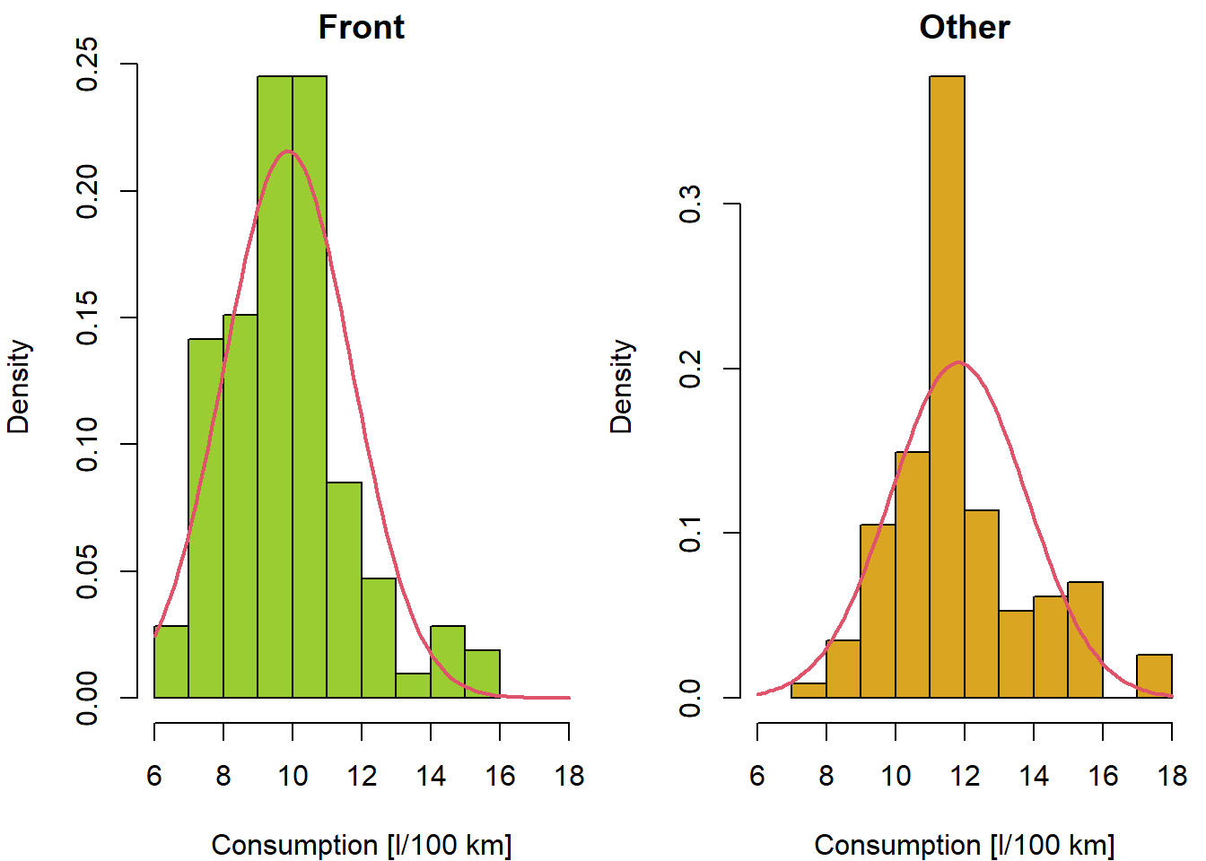
Histograms to inspect the shape of marginal distributions:
### Histograms
par(mfrow = c(1, 2), mar = c(4,4,0.5,0.5))
hist(Cars2004nh$consumption, prob = TRUE, main = "", col = "seagreen",
     xlab = "Consumption [l/100 km]")
hist(Cars2004nh$length, prob = TRUE, main = "", col = "seagreen",
     xlab = "Length [cm]")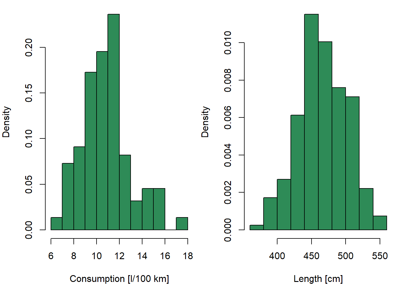
with(Cars2004nh, cor(consumption, length))## [1] NAwith(Cars2004nh, cor(consumption, length, use = "complete.obs"))## [1] 0.4311805with(Cars2004nh, cor(consumption, length, method = "spearman", use = "complete.obs"))## [1] 0.4562401Formal statistical test(s)
For each test refresh the following:
- What is the underlying model in each test?
- What are the assumptions?
Test based on Pearson’s correlation coefficient
with(Cars2004nh, cor.test(consumption, length))##
## Pearson's product-moment correlation
##
## data: consumption and length
## t = 6.7583, df = 200, p-value = 1.493e-10
## alternative hypothesis: true correlation is not equal to 0
## 95 percent confidence interval:
## 0.3116823 0.5372516
## sample estimates:
## cor
## 0.4311805Test based on Spearman’s correlation coefficient
with(Cars2004nh, cor.test(consumption, length, method = "spearman"))## Warning in cor.test.default(consumption, length, method = "spearman"): Cannot compute exact p-value with ties##
## Spearman's rank correlation rho
##
## data: consumption and length
## S = 746963, p-value = 8.869e-12
## alternative hypothesis: true rho is not equal to 0
## sample estimates:
## rho
## 0.4562401How would you assess the relationship between the dependent variable and independent covariates?
Here are some graphical tools to examine the (non)linearity of the relationship:
par(mfrow = c(1,1), mar = c(4,4,0.5,0.5))
plot(consumption ~ length, data = Cars2004nh, col = "red3", bg = "orange", pch = 23)
grid <- quantile(Cars2004nh$length, seq(0, 1, length = 20), na.rm = T)

xGrid <- NULL
yMean <- NULL
for(i in 2:length(grid)){
  tempData <- Cars2004nh$consumption[Cars2004nh$length >= grid[i - 1] & Cars2004nh$length < grid[i]]
  lines(rep(mean(tempData, na.rm = T), 2) ~ c(grid[i - 1], grid[i]), col = "red")
  points((grid[i - 1] + grid[i])/2, mean(tempData, na.rm = T),
         pch = 23, bg = "red", cex = 1.2)

  xGrid <- c(xGrid, (grid[i - 1] + grid[i])/2)
  yMean <- c(yMean, mean(tempData, na.rm = T))

  lines(rep(grid[i], 2), c(min(Cars2004nh$consumption), max(Cars2004nh$consumption)), lty = 3)
}
### which interpolates as:
lines(yMean ~ xGrid, col = "darkred", lwd = 3)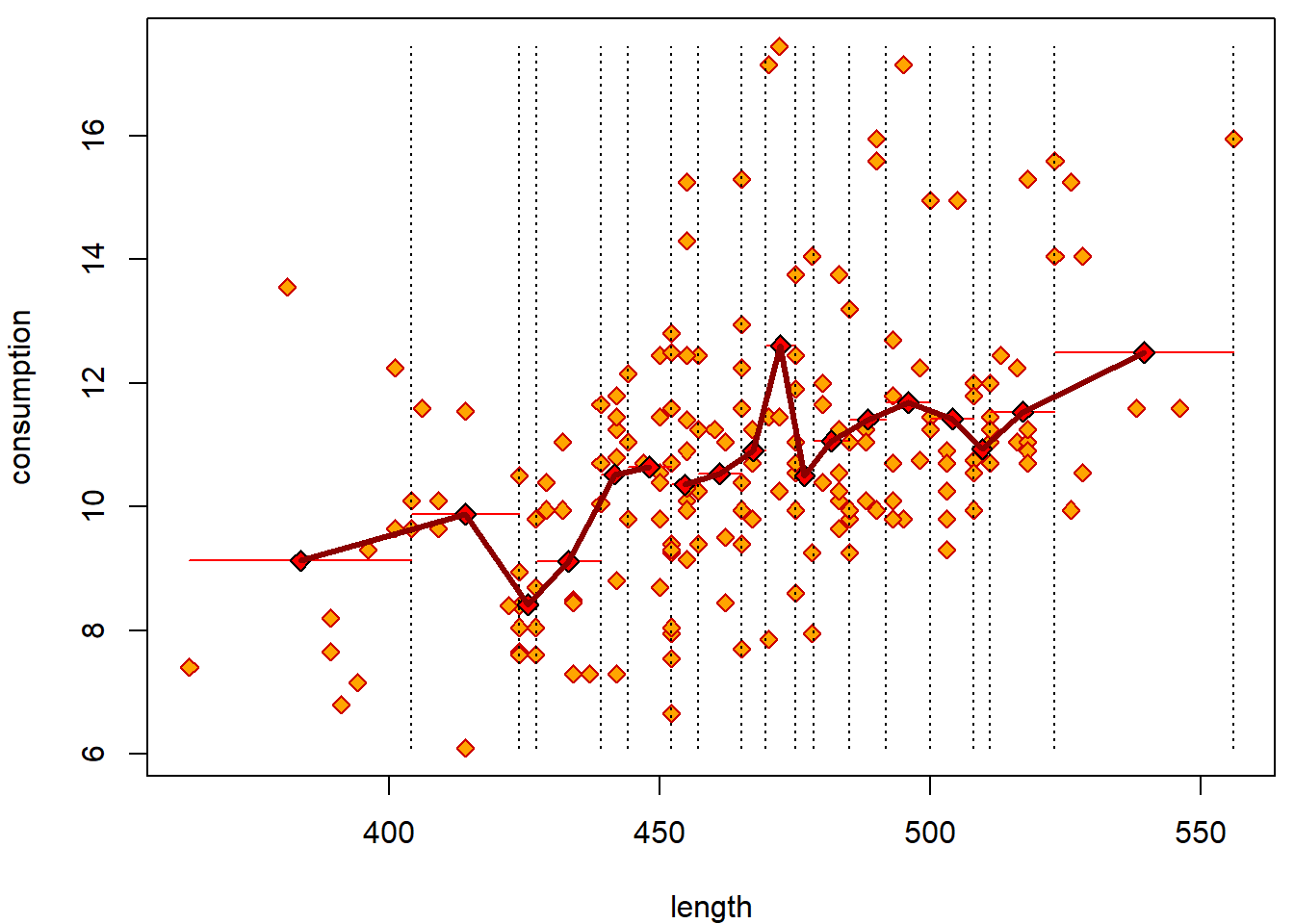
Less groups without for cycle:
grid <- quantile(Cars2004nh$length, seq(0, 1, length = 11), na.rm = T)
Cars2004nh$flength <- cut(Cars2004nh$length, breaks = grid, right = FALSE)
xGrid <- (grid[-1] + grid[-length(grid)]) / 2
yMean <- tapply(Cars2004nh$consumption, Cars2004nh$flength, mean)

par(mfrow = c(1,1), mar = c(4,4,0.5,0.5))
plot(consumption ~ length, data = Cars2004nh, type = "n")
segments(x0 = grid, y0 = min(Cars2004nh$consumption), y1 = max(Cars2004nh$consumption), lty = 3)
points(consumption ~ length, data = Cars2004nh, col = "red3", bg = "orange", pch = 23)
segments(x0 = grid[-length(grid)], x1 = grid[-1], y0 = yMean, col = "red")
lines(x = xGrid, y = yMean, col = "darkred", lwd = 3)
points(x = xGrid, y = yMean, pch = 23, bg = "red", cex = 1.2)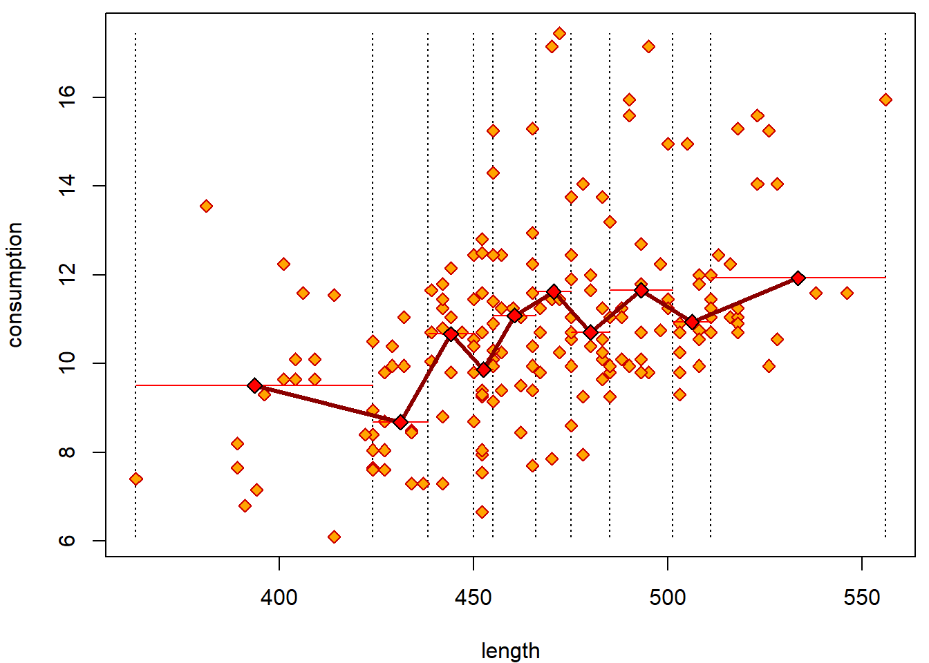
Category for every value of length that appears in the
data:
par(mfrow = c(1,1), mar = c(4,4,0.5,0.5))
plot(consumption ~ length, data = Cars2004nh, col = "red3", bg = "orange", pch = 23)
grid <- as.numeric(names(table(Cars2004nh$length)))
xGrid <- NULL
yMean <- NULL
for (i in 2:(length(grid) - 1)){
tempData <- Cars2004nh$consumption[Cars2004nh$length >= grid[i - 1] & Cars2004nh$length <= grid[i + 1]]
points(grid[i], mean(tempData, na.rm = T), pch = 23, bg = "red", cex = 1.2)
xGrid <- c(xGrid, grid[i])
yMean <- c(yMean, mean(tempData, na.rm = T))
}
### which now interpolates as:
lines(yMean ~ xGrid, col = "darkred", lwd = 3)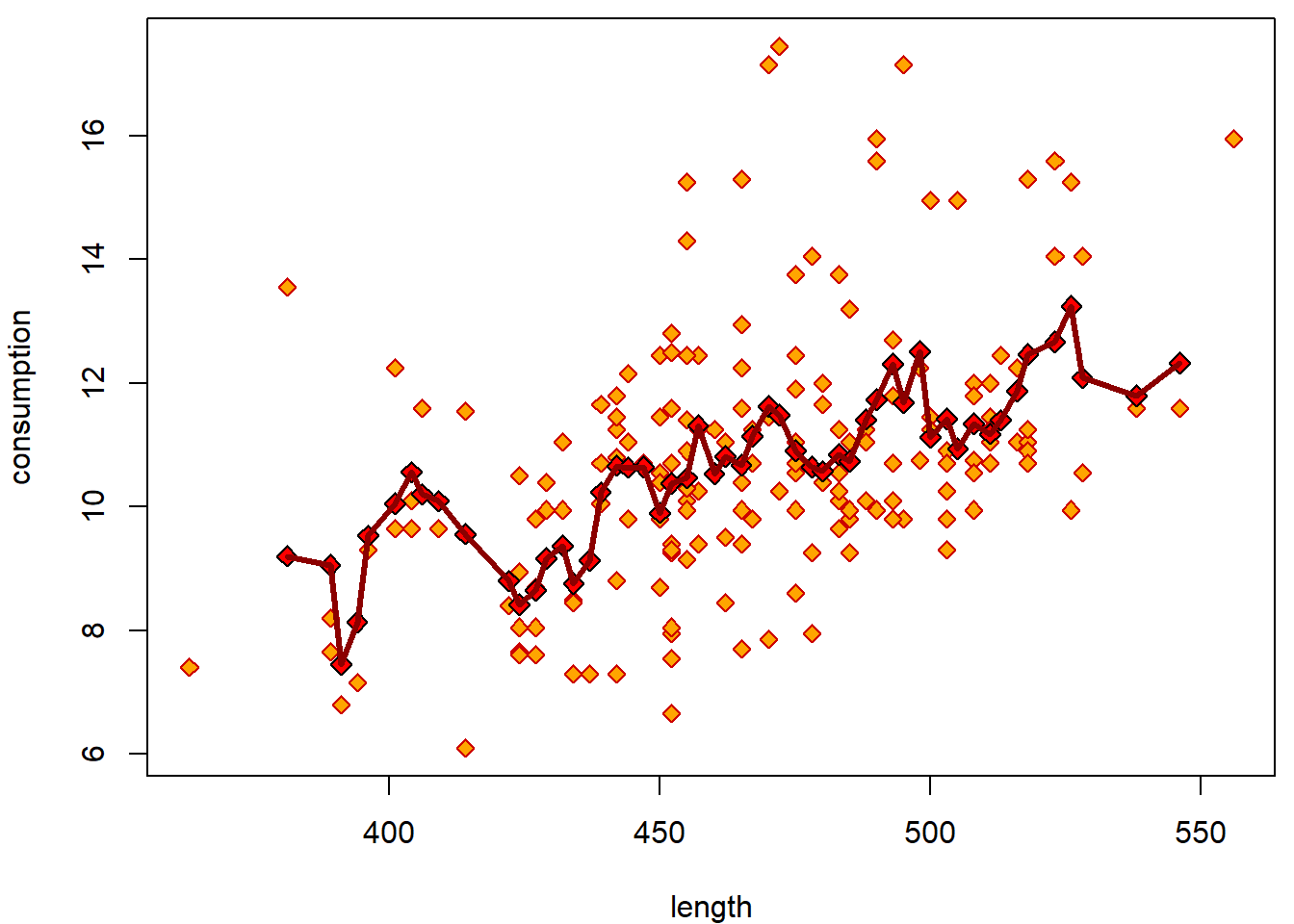 Local trend by
 lowess curve:
par(mfrow = c(1,3), mar = c(4,4,1.5,0.5))
for(f in c(1/10, 1/5, 1/2)){
plot(consumption ~ length, data = Cars2004nh, col = "red3", bg = "orange",
pch = 23, main = paste0("f = ", f))
tempData <- Cars2004nh[!is.na(Cars2004nh$length),]
lines(lowess(tempData$consumption ~ tempData$length, f = f), col = "red3", lwd = 3)
}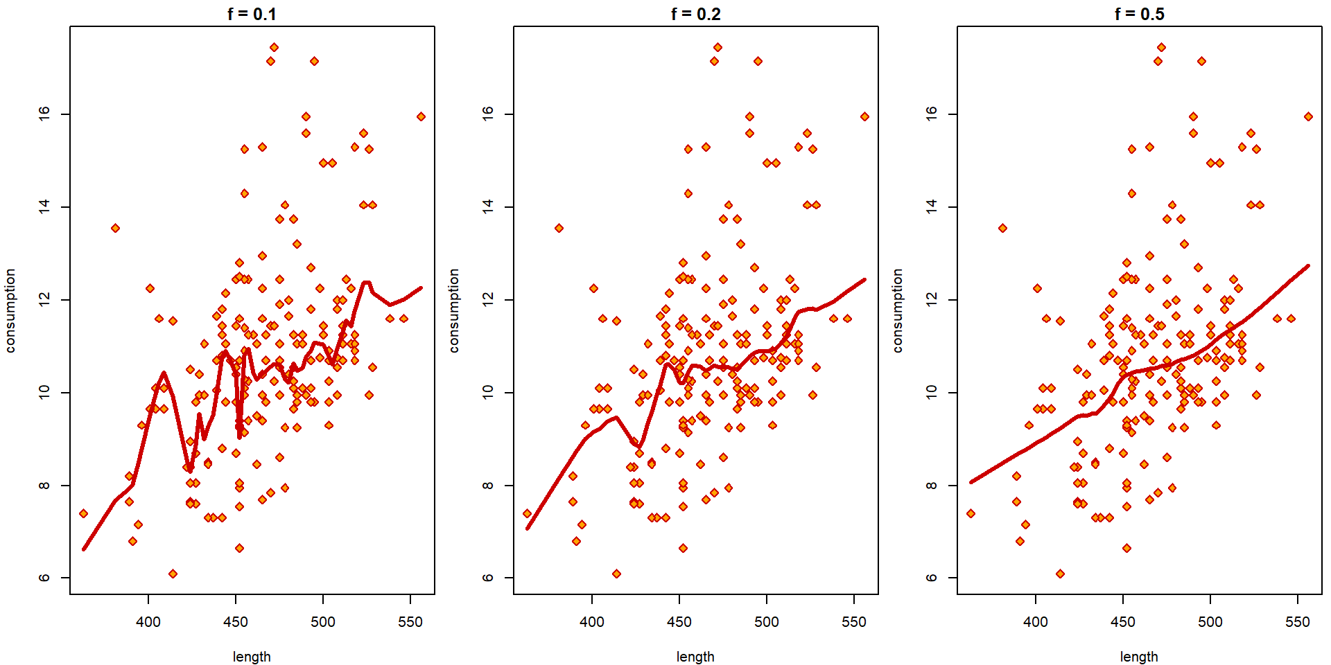 How a straight line should be fitted into the data?
Contingency table
We use them to capture the relationship between two categorical variables.
Does the fact that the car is economical (in the U.S. sense,
consumption <= 10) depend on the drive (distinguishing
only front and other)?
Exploration
The default plot for factor ~ factor is the spineplot
that compares the proportions of the first factor within each category
of the second factor separately:
par(mfrow = c(1,1), mar = c(4,4,1,2.5))
plot(fcons10 ~ fdrive2, data = Cars2004nh, col = diverge_hcl(2))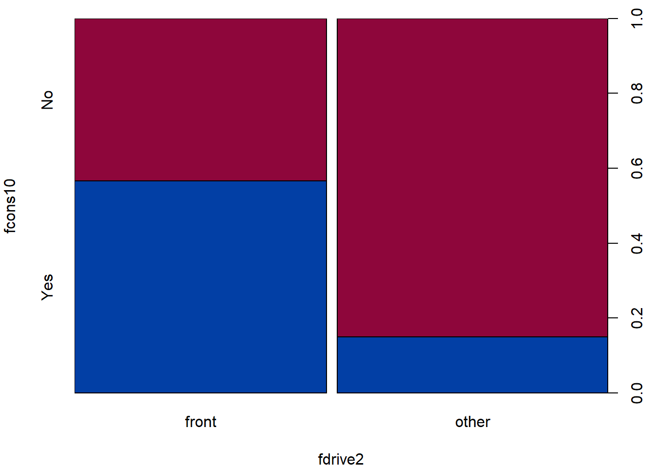
Contingency table:
(TAB2 <- with(Cars2004nh, table(fdrive2, fcons10)))## fcons10
## fdrive2 No Yes
## front 46 56
## other 98 20Proportion table:
round(prop.table(TAB2, margin = 1), 2)## fcons10
## fdrive2 No Yes
## front 0.45 0.55
## other 0.83 0.17Formal statistical test(s)
For each test refresh the following:
- What is the underlying model in each test?
- What are the assumptions?
Chi-square test using continuity correction to be more conservative
chisq.test(TAB2)##
## Pearson's Chi-squared test with Yates' continuity correction
##
## data: TAB2
## X-squared = 33.193, df = 1, p-value = 8.346e-09Chi-square test without continuity correction
(chi = chisq.test(TAB2, correct = FALSE))##
## Pearson's Chi-squared test
##
## data: TAB2
## X-squared = 34.851, df = 1, p-value = 3.559e-09How to obtain the test results manually:
# Expected observed counts under the null hypothesis
print(chi$expected)
## fcons10
## fdrive2 No Yes
## front 66.76364 35.23636
## other 77.23636 40.76364n = sum(TAB2) # number of observations
R = rowSums(TAB2)/n # observed proportion in rows
C = colSums(TAB2)/n # observed proportion in columns
n * outer(R, C) # expected counts under independence## No Yes
## front 66.76364 35.23636
## other 77.23636 40.76364(chi$observed - chi$expected)/sqrt(chi$expected) # residuals## fcons10
## fdrive2 No Yes
## front -2.541168 3.497904
## other 2.362613 -3.252123chi$residuals## fcons10
## fdrive2 No Yes
## front -2.541168 3.497904
## other 2.362613 -3.252123(ts<-sum(chi$res^2)) # test statistic## [1] 34.85111pchisq(ts, df=1, lower.tail=FALSE) # p-value## [1] 3.559067e-09Test based on difference between proportions. Notice the equivalency
to chisq.test. What can you learn from the output?
(x <- TAB2[, "Yes"])## front other
## 56 20(n <- apply(TAB2, 1, sum))## front other
## 102 118prop.test(x, n)##
## 2-sample test for equality of proportions with continuity correction
##
## data: x out of n
## X-squared = 33.193, df = 1, p-value = 8.346e-09
## alternative hypothesis: two.sided
## 95 percent confidence interval:
## 0.2524593 0.5065969
## sample estimates:
## prop 1 prop 2
## 0.5490196 0.1694915prop.test(x, n, correct = FALSE)##
## 2-sample test for equality of proportions without continuity correction
##
## data: x out of n
## X-squared = 34.851, df = 1, p-value = 3.559e-09
## alternative hypothesis: two.sided
## 95 percent confidence interval:
## 0.2615985 0.4974576
## sample estimates:
## prop 1 prop 2
## 0.5490196 0.1694915Reconstruction of the test statistic:
p2 = x/n              # proportion estimates in groups
p = sum(x) / sum(n)   # common proportion estimate
(ts <- (diff(p2) / sqrt(p*(1-p)*sum(1/n)))^2) # test statistic
## other
## 34.85111pchisq(ts, df=1, lower.tail=FALSE)## other
## 3.559067e-09What is tested here?
prop.test(x, n, alternative = "greater")##
## 2-sample test for equality of proportions with continuity correction
##
## data: x out of n
## X-squared = 33.193, df = 1, p-value = 4.173e-09
## alternative hypothesis: greater
## 95 percent confidence interval:
## 0.2714192 1.0000000
## sample estimates:
## prop 1 prop 2
## 0.5490196 0.1694915Individual work
Two sample problem
- Verify the assumptions for each two-sample test.
- For instance, a formal test for equal variances in two groups or visual assessment of normality of the two samples.
- How would you visualize the sample means and medians which are tested in the two-sample problems?
More sample problem
- Instead of using three group specific means, consider a reformulation by using the conditional mean given the groups. What is the analogy with the regression formulation?
Contingency tables
- Try also for categorical variables with more than 2 groups.
- Explore the following pairs: (
fcons10,fdrive) and (fdrive,ftype).
For practical purposes one sided alternative can be tested instead. Which alternative makes more sense? What exactly do we test here? Reconstruct the test statistics and the corresponding p-values.
t.test(consumption ~ fdrive2, data = Cars2004nh, alternative = "less", mu = -2)##
## Welch Two Sample t-test
##
## data: consumption by fdrive2
## t = -0.27403, df = 217.59, p-value = 0.3922
## alternative hypothesis: true difference in means between group front and group other is less than -2
## 95 percent confidence interval:
## -Inf -1.633921
## sample estimates:
## mean in group front mean in group other
## 9.866176 11.938983t.test(consumption ~ fdrive2, data = Cars2004nh, alternative = "less", mu = -2,
var.equal = TRUE)##
## Two Sample t-test
##
## data: consumption by fdrive2
## t = -0.27198, df = 218, p-value = 0.3929
## alternative hypothesis: true difference in means between group front and group other is less than -2
## 95 percent confidence interval:
## -Inf -1.63062
## sample estimates:
## mean in group front mean in group other
## 9.866176 11.938983wilcox.test(consumption ~ fdrive2, data = Cars2004nh, alternative = "less",
mu = -2, conf.int = TRUE)##
## Wilcoxon rank sum test with continuity correction
##
## data: consumption by fdrive2
## W = 6253, p-value = 0.6916
## alternative hypothesis: true location shift is less than -2
## 95 percent confidence interval:
## -Inf -1.449976
## sample estimates:
## difference in location
## -1.89995Does the fact that the car is economical (in the U.S. sense,
consumption<=10) depend on the drive (while
distinguishing front, rear or
4x4)?
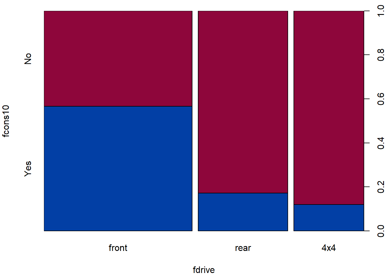
- What are we testing by the following test?
- What is the model behind this test?
- Does the model seem to be good enough to be useful?
- Which artefacts of the model might be relatively safely ignored and why?
- What is the conclusion?
chisq.test(TAB3)##
## Pearson's Chi-squared test
##
## data: TAB3
## X-squared = 35.914, df = 2, p-value = 1.59e-08print(chisq.test(TAB3)$expected)## fcons10
## fdrive No Yes
## front 66.76364 35.23636
## rear 39.92727 21.07273
## 4x4 37.30909 19.69091print(chisq.test(TAB3)$residuals)## fcons10
## fdrive No Yes
## front -2.541168 3.497904
## rear 1.277572 -1.758571
## 4x4 2.077712 -2.859959print(chisq.test(TAB3)$stdres)## fcons10
## fdrive No Yes
## front -5.903483 5.903483
## rear 2.556835 -2.556835
## 4x4 4.106837 -4.106837Does the drive (front/rear/4x4) depend on the type of the car (personal/wagon/SUV/pickup/sport/minivan)?
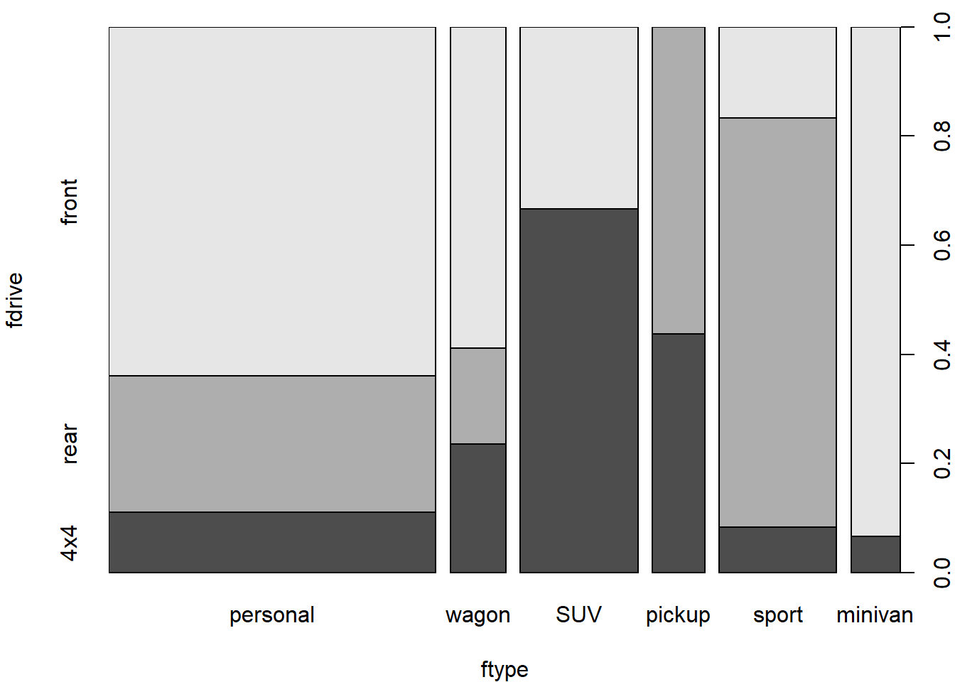
- What are we testing by the following test?
- What is the model behind this test?
- Does the model seem to be good enough to be useful?
- Which artefacts of the model might be relatively safely ignored and why?
- What is the conclusion?
- Why did we get the warning message? What can be done about it?
chisq.test(TAB4)## Warning in chisq.test(TAB4): Chi-squared approximation may be incorrect##
## Pearson's Chi-squared test
##
## data: TAB4
## X-squared = 110.76, df = 10, p-value < 2.2e-16print(chisq.test(TAB4)$expected)## Warning in chisq.test(TAB4): Chi-squared approximation may be incorrect## fdrive
## ftype front rear 4x4
## personal 46.363636 27.727273 25.909091
## wagon 8.809091 5.268182 4.922727
## SUV 19.009091 11.368182 10.622727
## pickup 8.345455 4.990909 4.663636
## sport 13.445455 8.040909 7.513636
## minivan 6.027273 3.604545 3.368182