Heteroscedastic models
Jan Vávra
Exercise 10
Download this R markdown as: R, Rmd.
Outline of this lab session:
- Statistical inference in heteroscedastic model
- General linear model (known variance structure)
- Heteroscedastic model with unknown structure
The idea is to consider a general version of the linear regression model where \[ \boldsymbol{Y} \sim \mathsf{N}(\mathbb{X}\boldsymbol{\beta}, \sigma^2 \mathbb{W}^{-1}), \] where \(\boldsymbol{Y} = (Y_1, \dots, Y_n)^\top\) is the response vector for \(n \in \mathbb{N}\) independent subjects, \(\mathbb{X}\) is the corresponding model matrix (of a full rank \(p \in \mathbb{N}\)) and \(\boldsymbol{\beta} \in \mathbb{R}^p\) is the vector of the unknown parameters.
Note, that the normality assumption above is only used as a simplification but it is not needed to fit the model (without normality the results and the inference will hold asymptotically).
Considering the variance structure, reflected in the matrix \(\mathbb{W} \in \mathbb{R}^{n \times n}\) (a diagonal matrix because the subjects are mutually independent) can distinguish two cases:
- the variance matrix \(\mathbb{W}\) is a known matrix,
- the variance matrix \(\mathbb{W}\) is an unknown matrix.
These cases lead to the so-called
- general linear model (not a generalized linear model, which is a different class of models)
- and a regression model under heteroscedastic errors.
Both cases will be briefly addressed below.
1. General linear model
library("mffSM")        # Hlavy, plotLM()
library("colorspace")   # color palettes
library("MASS")         # sdres()
library("sandwich")     # vcovHC()
library("lmtest")       # coeftest()
data(Hlavy, package = "mffSM")
We start with the dataset Hlavy (heads) which represents
head sizes of fetuses (from an ultrasound monitoring) in different
periods of pregnancy. Each data value (row in the dataframe) provides an
average over \(n_i \in \mathbb{N}\)
measurements of \(n_i\) independent
subjects (mothers).
The information provided in the data stand for the:
iserial number,tweek of the pregnancy,nnumber of measurements used to calculate the average head size,ythe average head size obtained from the particular number of measurements.
head(Hlavy)## i t n y
## 1 1 16 2 5.100
## 2 2 18 3 5.233
## 3 3 19 9 4.744
## 4 4 20 10 5.110
## 5 5 21 11 5.236
## 6 6 22 20 5.740dim(Hlavy)## [1] 26 4summary(Hlavy)## i t n y
## Min. : 1.00 Min. :16.00 Min. : 2.00 Min. :4.744
## 1st Qu.: 7.25 1st Qu.:23.25 1st Qu.:20.25 1st Qu.:5.871
## Median :13.50 Median :29.50 Median :47.00 Median :7.776
## Mean :13.50 Mean :29.46 Mean :39.85 Mean :7.461
## 3rd Qu.:19.75 3rd Qu.:35.75 3rd Qu.:60.00 3rd Qu.:8.980
## Max. :26.00 Max. :42.00 Max. :85.00 Max. :9.633par(mfrow = c(1,1), mar = c(4,4,0.5,0.5))
plot(y ~ t, data = Hlavy, pch = 23, col = "red3", bg = "orange")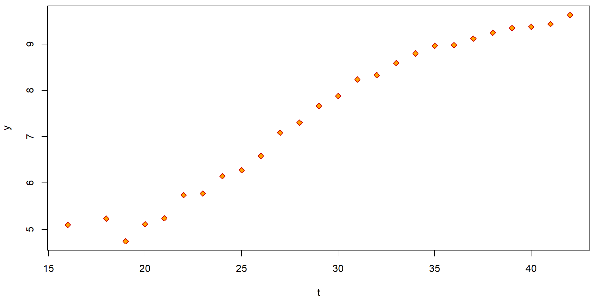
The simple scatterplot above can be, however, substantially improved by accounting also for reliability of each observation (higher number of measurements used to obtain the average also means higher reliability). This can be obtain, for instance, by the following code:
with(Hlavy, quantile(n, prob = seq(0, 1, by = 0.2)))## 0% 20% 40% 60% 80% 100%
## 2 11 31 53 60 85Hlavy <- transform(Hlavy,
fn = cut(n, breaks = c(0, 10, 30, 50, 60, 90),
labels = c("<=10", "11-30", "31-50", "51-60", ">60")),
cexn = n/25+1)
with(Hlavy, summary(fn))## <=10 11-30 31-50 51-60 >60
## 5 5 5 6 5plotHlavy <- function(){
PAL <- rev(heat_hcl(nlevels(Hlavy[, "fn"]), c.=c(80, 30), l=c(30, 90), power=c(1/5, 1.3)))
names(PAL) <- levels(Hlavy[, "fn"])
plot(y ~ t, data = Hlavy,
xlab = "Week", ylab = "Average head size",
pch = 23, col = "black", bg = PAL[fn], cex = cexn)
legend(17, 9, legend = levels(Hlavy[, "fn"]), title = "n", fill = PAL)
abline(v = 27, col = "lightblue", lty = 2)
}
par(mfrow = c(1,1), mar = c(4,4,0.5,0.5))
plotHlavy()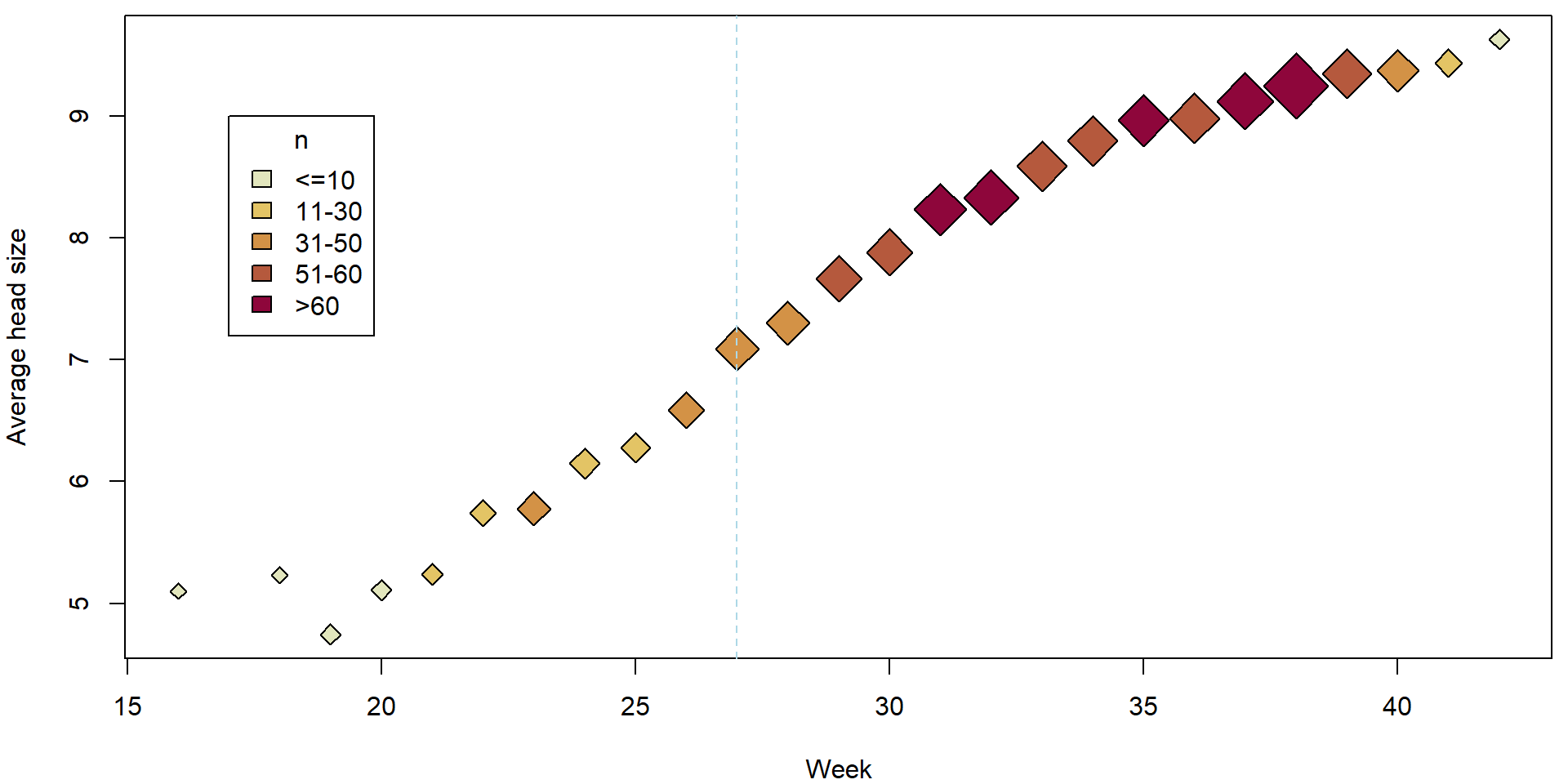
It is reasonable to assume, that for each independent measurement \(\widetilde{Y}_{ij}\) we have some model of the form \[ \widetilde{Y}_{ij} | \boldsymbol{X}_{i} \sim \mathsf{N}(\boldsymbol{X}_{i}^\top\boldsymbol{\beta}, \sigma^2) \] where for each \(j \in \{1, \ldots, n_i\}\) these observations are measured under the same set of covariates \(\mathbf{X_i}\). This is a homoscedastic model.
Unfortunately, we do not observe \(\widetilde{Y}_{ij}\) directly, but, instead, we only observe the overall average \(Y_i = \frac{1}{n_i}\sum_{j = 1}^{n_i} \widetilde{Y}_{ij}\).
It also holds, that \[ Y_i \sim \mathsf{N}(\boldsymbol{X}_i^\top\boldsymbol{\beta}, \sigma^2/{n_i}), \] or, considering all data together, we have \[ \boldsymbol{Y} \sim \mathsf{N}_n(\mathbb{X}\boldsymbol{\beta}, \sigma^2 \mathbb{W}^{-1}), \] where \(\mathbb{W}^{-1}\) is a diagonal matrix \(\mathbb{W}^{-1} = \mathsf{diag}(1/n_1, \dots, 1/n_n)\) (thus, the variance structure is known from the design of the experiment). The matrix \(\mathbb{W} = \mathsf{diag}(n_1, \dots, n_n)\) is the weight matrix which gives each \(Y_i\) the weight corresponding to number of observations it has been obtained from.
In addition, practical motivation behind the model is the following:
Practitioners say that the relationship y ~ t could be
described by a piecewise quadratic function with t = 27
being a point where the quadratic relationship changes its shape.
From the practical point of view, the fitted curve should be
continuous at t = 27 and perhaps also
smooth (i.e., with continuous at least the first
derivative) as it is biologically not defensible to claim that at
t = 27 the growth has a jump in the speed (rate) of the
growth.
As far as different observations have different credibility, we will use the general linear model with the known matrix \(\mathbb{W}\). The model can be fitted as follows:
Hlavy <- transform(Hlavy, t27 = t - 27)

summary(mCont <- lm(y ~ t27 + I(t27^2) + (t27 > 0):t27 + (t27 > 0):I(t27^2),
                    weights = n, data = Hlavy))
##
## Call:
## lm(formula = y ~ t27 + I(t27^2) + (t27 > 0):t27 + (t27 > 0):I(t27^2),
## data = Hlavy, weights = n)
##
## Weighted Residuals:
## Min 1Q Median 3Q Max
## -0.88212 -0.35216 0.01232 0.37917 0.85320
##
## Coefficients:
## Estimate Std. Error t value Pr(>|t|)
## (Intercept) 7.049749 0.042425 166.170 < 2e-16 ***
## t27 0.381177 0.030288 12.585 3.01e-11 ***
## I(t27^2) 0.016214 0.003943 4.112 0.000497 ***
## t27:t27 > 0TRUE -0.063531 0.039426 -1.611 0.122017
## I(t27^2):t27 > 0TRUE -0.026786 0.003776 -7.094 5.35e-07 ***
## ---
## Signif. codes: 0 '***' 0.001 '**' 0.01 '*' 0.05 '.' 0.1 ' ' 1
##
## Residual standard error: 0.477 on 21 degrees of freedom
## Multiple R-squared: 0.9968, Adjusted R-squared: 0.9962
## F-statistic: 1652 on 4 and 21 DF, p-value: < 2.2e-16Compare to the naive (and incorrect) model where the weights are ignored:
mCont_noweights <- lm(y ~ t27 + I(t27^2) + (t27 > 0):t27 + (t27 > 0):I(t27^2), data = Hlavy)
summary(mCont_noweights)
##
## Call:
## lm(formula = y ~ t27 + I(t27^2) + (t27 > 0):t27 + (t27 > 0):I(t27^2),
## data = Hlavy)
##
## Residuals:
## Min 1Q Median 3Q Max
## -0.34389 -0.05749 -0.01730 0.05353 0.22852
##
## Coefficients:
## Estimate Std. Error t value Pr(>|t|)
## (Intercept) 7.084353 0.069011 102.655 < 2e-16 ***
## t27 0.422937 0.032626 12.963 1.73e-11 ***
## I(t27^2) 0.021672 0.003110 6.968 7.00e-07 ***
## t27:t27 > 0TRUE -0.121159 0.049259 -2.460 0.0227 *
## I(t27^2):t27 > 0TRUE -0.030978 0.002924 -10.593 7.00e-10 ***
## ---
## Signif. codes: 0 '***' 0.001 '**' 0.01 '*' 0.05 '.' 0.1 ' ' 1
##
## Residual standard error: 0.1212 on 21 degrees of freedom
## Multiple R-squared: 0.9955, Adjusted R-squared: 0.9947
## F-statistic: 1173 on 4 and 21 DF, p-value: < 2.2e-16Fitted curves:
tgrid <- seq(16, 42, length = 100)
pdata <- data.frame(t27 = tgrid - 27)
fitCont <- predict(mCont, newdata = pdata)

par(mfrow = c(1,1), mar = c(4,4,0.5,0.5))
plotHlavy()
lines(tgrid, fitCont, col = "red2", lwd = 3)
lines(tgrid, predict(mCont_noweights, newdata = pdata), col = "navyblue", lwd = 2, lty = 2)
legend("bottomright", bty = "n",
       legend = c(bquote(Weights: hat(sigma) == .(summary(mCont)$sigma)),
                  bquote(Noweights: hat(sigma) == .(summary(mCont_noweights)$sigma))),
       col = c("red2", "navyblue"), lty = c(1,2), lwd = c(2,3))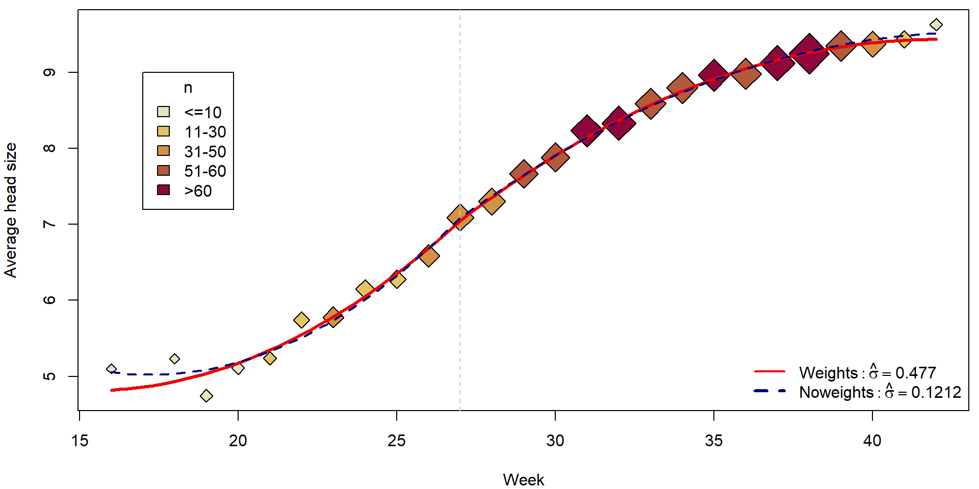
Individual work
- What is estimated by the model above? Interpret the estimated parameters.
- Can you manually reconstruct the estimated values for the mean structure and, also, the estimated values for the variance parameters?
### Key matrices
W <- diag(Hlavy$n)
Y <- Hlavy$y
X <- model.matrix(mCont)

### Estimated regression coefficients
c(betahat <- solve(t(X) %*% W %*% X) %*% (t(X) %*% W %*% Y))
## [1] 7.04974918 0.38117667 0.01621412 -0.06353122 -0.02678567coef(mCont)## (Intercept) t27 I(t27^2) t27:t27 > 0TRUE I(t27^2):t27 > 0TRUE
## 7.04974918 0.38117667 0.01621412 -0.06353122 -0.02678567### Generalized fitted values
c(Yg <- X %*% betahat)## [1] 4.818714 4.932503 5.038040 5.176004 5.346398 5.549219 5.784468 6.052146 6.352252 6.684787 7.049749
## [12] 7.356823 7.642754 7.907542 8.151186 8.373688 8.575046 8.755262 8.914334 9.052263 9.169049 9.264692
## [23] 9.339192 9.392549 9.424762 9.435833fitted(mCont)## 1 2 3 4 5 6 7 8 9 10 11 12
## 4.818714 4.932503 5.038040 5.176004 5.346398 5.549219 5.784468 6.052146 6.352252 6.684787 7.049749 7.356823
## 13 14 15 16 17 18 19 20 21 22 23 24
## 7.642754 7.907542 8.151186 8.373688 8.575046 8.755262 8.914334 9.052263 9.169049 9.264692 9.339192 9.392549
## 25 26
## 9.424762 9.435833### Generalized residual sum of squares
(RSS <- t(Y - Yg) %*% W %*% (Y - Yg))## [,1]
## [1,] 4.777559### Generalized mean square
RSS/(length(Y)-ncol(X))## [,1]
## [1,] 0.2275028(summary(mCont)$sigma)^2## [1] 0.2275028### Be careful that Multiple R-squared: 0.9968 reported in the output "summary(mCont)" is not equal to
sum((Yg-mean(Yg))^2)/sum((Y-mean(Y))^2)## [1] 1.005601### Instead, it equals the following quantity that is more difficult to interpret
barYw <- sum(Y*Hlavy$n)/sum(Hlavy$n)
### weighted mean of the original observations
### something as "generalized" regression sum of squares
SSR <- sum((Yg - barYw)^2 * Hlavy$n)
### something as "generalized" total variance
SST <- sum((Y - barYw)^2 * Hlavy$n)
### "generalized" R squared
SSR/SST## [1] 0.9968318summary(mCont)$r.squared## [1] 0.9968318- Compare the general linear model above with the simple model below. What are the main differences between these two models? Can you explain them?
iii <- rep(1:nrow(Hlavy), Hlavy$n)
Hlavy2 <- Hlavy[iii,] # new dataset

summary(mCont2 <- lm(y ~ t27 + I(t27^2) + (t27 > 0):t27 + (t27 > 0):I(t27^2), data = Hlavy2))
##
## Call:
## lm(formula = y ~ t27 + I(t27^2) + (t27 > 0):t27 + (t27 > 0):I(t27^2),
## data = Hlavy2)
##
## Residuals:
## Min 1Q Median 3Q Max
## -0.29404 -0.04505 -0.01469 0.04125 0.30050
##
## Coefficients:
## Estimate Std. Error t value Pr(>|t|)
## (Intercept) 7.0497492 0.0060548 1164.32 <2e-16 ***
## t27 0.3811767 0.0043227 88.18 <2e-16 ***
## I(t27^2) 0.0162141 0.0005628 28.81 <2e-16 ***
## t27:t27 > 0TRUE -0.0635312 0.0056268 -11.29 <2e-16 ***
## I(t27^2):t27 > 0TRUE -0.0267857 0.0005389 -49.70 <2e-16 ***
## ---
## Signif. codes: 0 '***' 0.001 '**' 0.01 '*' 0.05 '.' 0.1 ' ' 1
##
## Residual standard error: 0.06807 on 1031 degrees of freedom
## Multiple R-squared: 0.9968, Adjusted R-squared: 0.9968
## F-statistic: 8.11e+04 on 4 and 1031 DF, p-value: < 2.2e-16summary(mCont)##
## Call:
## lm(formula = y ~ t27 + I(t27^2) + (t27 > 0):t27 + (t27 > 0):I(t27^2),
## data = Hlavy, weights = n)
##
## Weighted Residuals:
## Min 1Q Median 3Q Max
## -0.88212 -0.35216 0.01232 0.37917 0.85320
##
## Coefficients:
## Estimate Std. Error t value Pr(>|t|)
## (Intercept) 7.049749 0.042425 166.170 < 2e-16 ***
## t27 0.381177 0.030288 12.585 3.01e-11 ***
## I(t27^2) 0.016214 0.003943 4.112 0.000497 ***
## t27:t27 > 0TRUE -0.063531 0.039426 -1.611 0.122017
## I(t27^2):t27 > 0TRUE -0.026786 0.003776 -7.094 5.35e-07 ***
## ---
## Signif. codes: 0 '***' 0.001 '**' 0.01 '*' 0.05 '.' 0.1 ' ' 1
##
## Residual standard error: 0.477 on 21 degrees of freedom
## Multiple R-squared: 0.9968, Adjusted R-squared: 0.9962
## F-statistic: 1652 on 4 and 21 DF, p-value: < 2.2e-162. Model with heteroscedastic errors (sandwich estimate)
For a general heteroscedastic model it is usually
assumed that
\[
Y_i | \boldsymbol{X}_i \sim
\mathsf{N}(\boldsymbol{X}_i^\top\boldsymbol{\beta},
\sigma^2(\boldsymbol{X}_i))
\] where \(\sigma^2(\cdot)\) is
some positive (unknown) function of the response variables \(\boldsymbol{X}_i \in \mathbb{R}^p\). Note,
that the normality assumption is here only given for simplification but
it is not required.
In the following, we will consider the dataset that comes from the
project MANA (Maturita na necisto) launched in the Czech Republic in
2005. This project was a part of a bigger project whose goal was to
prepare a new form of graduation exam (“statni maturita”).
This dataset contains the results in English language at grammar
schools.
load(url("http://msekce.karlin.mff.cuni.cz/~vavraj/nmfm334/data/mana.RData"))The variables in the data are:
region(1 = Praha; 2 = Stredocesky; 3 = Jihocesky; 4 = Plzensky; 5 = Karlovarsky; 6 = Ustecky; 7 = Liberecky; 8 = Kralovehradecky; 9 = Pardubicky; 10 = Vysocina; 11 = Jihomoravsky; 12 = Olomoucky; 13 = Zlinsky; 14 = Moravskoslezsky),specialization(1 = education; 2 = social science; 3 = languages; 4 = law; 5 = math-physics; 6 = engineering; 7 = science; 8 = medicine; 9 = economics; 10 = agriculture; 11 = art),gender(0 = female; 1 = male),graduation(0 = no; 1 = yes),entry.exam(0 = no; 1 = yes),score(score in English language in MANA test),avg.mark(average mark (grade) from all subjects at the last report card), andmark.eng(average mark (grade) from the English language at the last 5 report cards).
For better intuition, we can transform the data as follows:
mana <- transform(mana,
                  fregion = factor(region, levels = 1:14,
                                   labels = c("A", "S", "C", "P", "K", "U", "L",
                                              "H", "E", "J", "B", "M", "Z", "T")),
                  fspec = factor(specialization, levels = 1:11,
                                 labels = c("Educ", "Social", "Lang", "Law",
                                            "Mat-Phys", "Engin", "Science",
                                            "Medic", "Econom", "Agric", "Art")),
                  fgender = factor(gender, levels = 0:1, labels = c("Female", "Male")),
                  fgrad = factor(graduation, levels = 0:1, labels = c("No", "Yes")),
                  fentry  = factor(entry.exam, levels = 0:1,  labels = c("No", "Yes")))

summary(mana)
## region specialization gender graduation entry.exam score
## Min. : 1.000 Min. : 1.000 Min. :0.000 Min. :0.0000 Min. :0.0000 Min. : 5.00
## 1st Qu.: 3.000 1st Qu.: 2.000 1st Qu.:0.000 1st Qu.:1.0000 1st Qu.:0.0000 1st Qu.:40.00
## Median : 7.000 Median : 6.000 Median :0.000 Median :1.0000 Median :0.0000 Median :44.00
## Mean : 7.462 Mean : 5.496 Mean :0.415 Mean :0.9585 Mean :0.4536 Mean :43.02
## 3rd Qu.:11.000 3rd Qu.: 8.000 3rd Qu.:1.000 3rd Qu.:1.0000 3rd Qu.:1.0000 3rd Qu.:48.00
## Max. :14.000 Max. :11.000 Max. :1.000 Max. :1.0000 Max. :1.0000 Max. :52.00
##
## avg.mark mark.eng fregion fspec fgender fgrad fentry
## Min. :1.000 Min. :1.000 T : 923 Social : 855 Female:3044 No : 216 No :2843
## 1st Qu.:1.480 1st Qu.:1.400 S : 665 Econom : 846 Male :2159 Yes:4987 Yes:2360
## Median :1.640 Median :2.000 B : 634 Engin : 638
## Mean :1.645 Mean :2.176 A : 599 Medic : 564
## 3rd Qu.:1.810 3rd Qu.:2.800 L : 534 Science: 557
## Max. :2.470 Max. :4.200 C : 474 Educ : 513
## (Other):1374 (Other):1230Individual work
- Consider the transformed data above and perform a simple exploratory analysis (in terms of some simple sample characteristics and plots).
- Focus, in particular on the region in the Czech republic and the specialization.
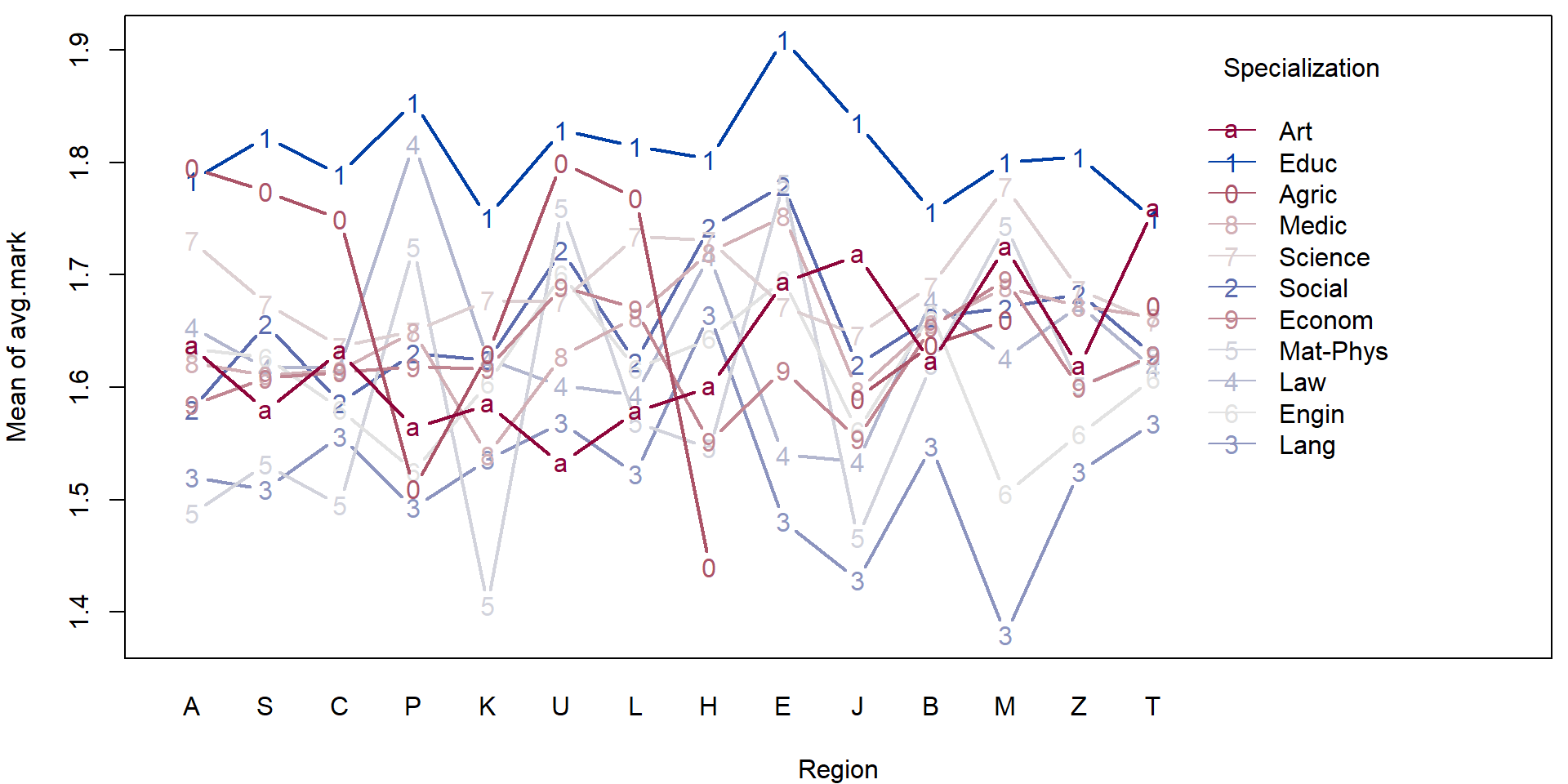
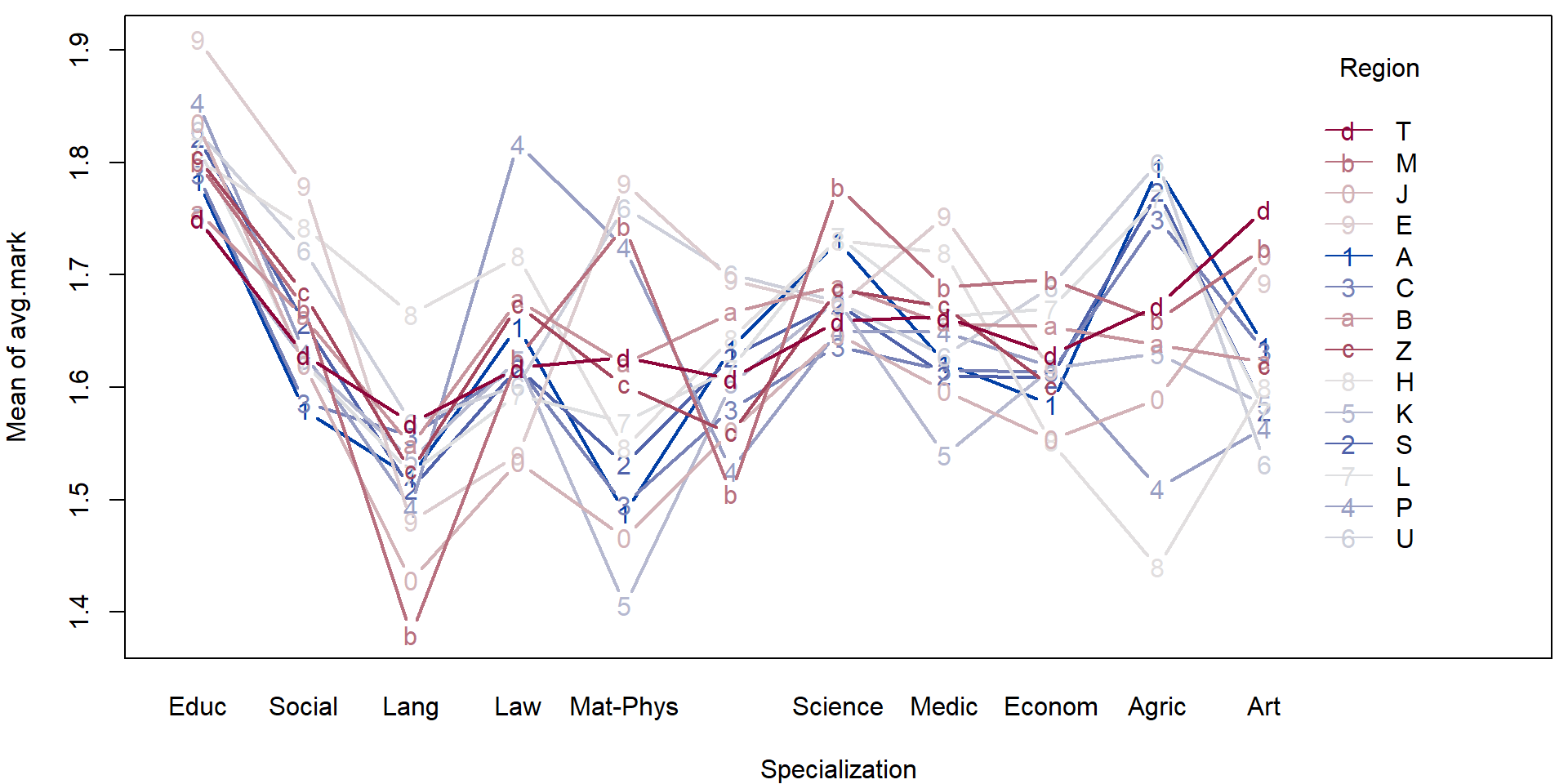
For illustration purposes we will fit a simple (additive) model to explain the average mark given the region and the specialization.
mAddit <- lm(avg.mark ~ fregion + fspec, data = mana)
summary(mAddit)
##
## Call:
## lm(formula = avg.mark ~ fregion + fspec, data = mana)
##
## Residuals:
## Min 1Q Median 3Q Max
## -0.68845 -0.16441 -0.00517 0.15618 0.84024
##
## Coefficients:
## Estimate Std. Error t value Pr(>|t|)
## (Intercept) 1.77616 0.01432 124.065 < 2e-16 ***
## fregionS 0.00887 0.01334 0.665 0.5063
## fregionC -0.01336 0.01455 -0.918 0.3585
## fregionP 0.02008 0.02197 0.914 0.3607
## fregionK -0.02198 0.02098 -1.048 0.2948
## fregionU 0.05678 0.02049 2.772 0.0056 **
## fregionL 0.02388 0.01411 1.692 0.0907 .
## fregionH 0.04861 0.02104 2.310 0.0209 *
## fregionE 0.07980 0.02049 3.894 9.98e-05 ***
## fregionJ -0.03138 0.01942 -1.616 0.1062
## fregionB 0.03236 0.01348 2.400 0.0164 *
## fregionM 0.02588 0.02159 1.199 0.2306
## fregionZ 0.01653 0.01880 0.879 0.3794
## fregionT 0.00846 0.01250 0.677 0.4984
## fspecSocial -0.15080 0.01325 -11.382 < 2e-16 ***
## fspecLang -0.26387 0.01700 -15.520 < 2e-16 ***
## fspecLaw -0.15020 0.01534 -9.789 < 2e-16 ***
## fspecMat-Phys -0.22192 0.01926 -11.525 < 2e-16 ***
## fspecEngin -0.17752 0.01403 -12.655 < 2e-16 ***
## fspecScience -0.10411 0.01448 -7.191 7.36e-13 ***
## fspecMedic -0.14369 0.01446 -9.938 < 2e-16 ***
## fspecEconom -0.16751 0.01330 -12.591 < 2e-16 ***
## fspecAgric -0.07115 0.03120 -2.281 0.0226 *
## fspecArt -0.15527 0.02030 -7.650 2.38e-14 ***
## ---
## Signif. codes: 0 '***' 0.001 '**' 0.01 '*' 0.05 '.' 0.1 ' ' 1
##
## Residual standard error: 0.236 on 5179 degrees of freedom
## Multiple R-squared: 0.07124, Adjusted R-squared: 0.06712
## F-statistic: 17.27 on 23 and 5179 DF, p-value: < 2.2e-16par(mar = c(4,4,1.5,0.5))
plotLM(mAddit)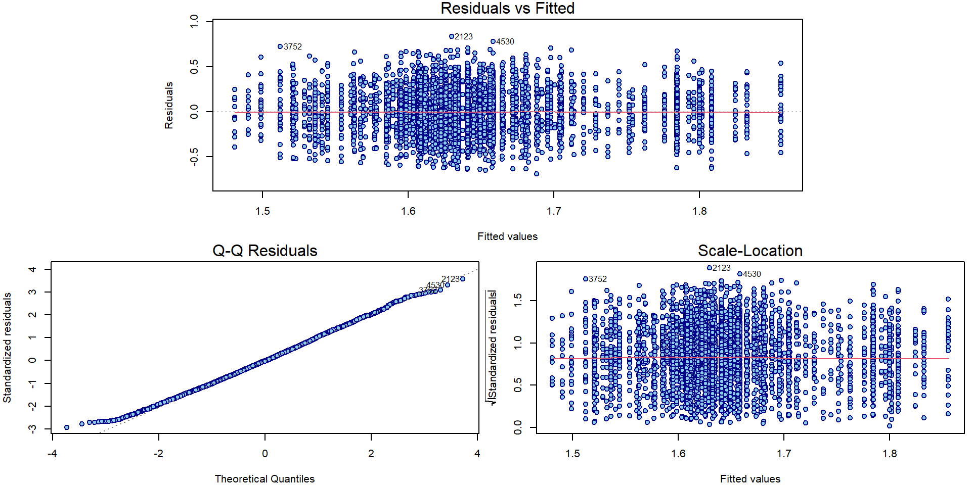 Could the variability vary with the region or school specialization?
par(mfrow = c(1,1), mar = c(4,4,0.5,0.5))
plot(sqrt(abs(stdres(mAddit))) ~ mana$fregion)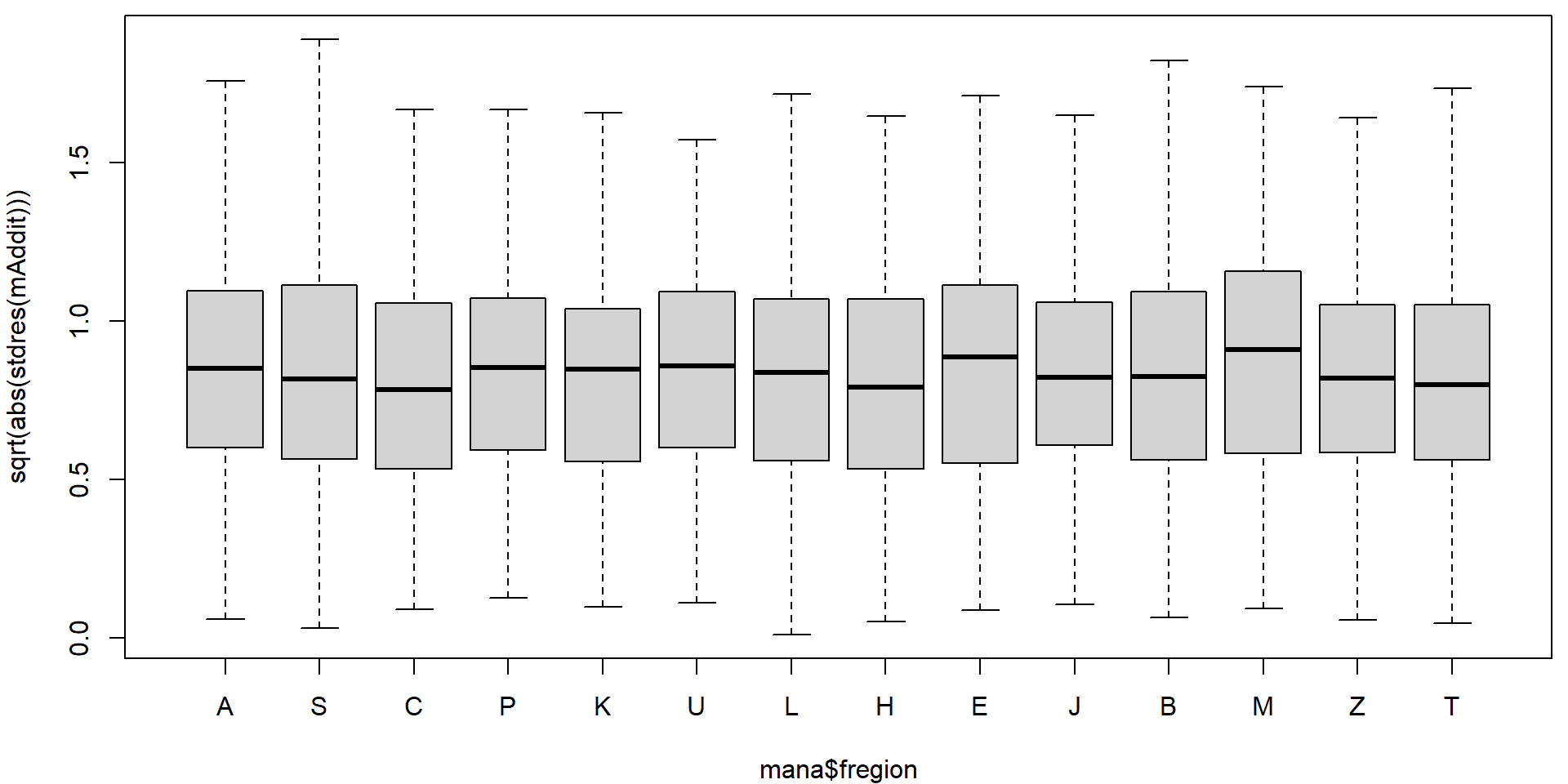
plot(sqrt(abs(stdres(mAddit))) ~ mana$fspec)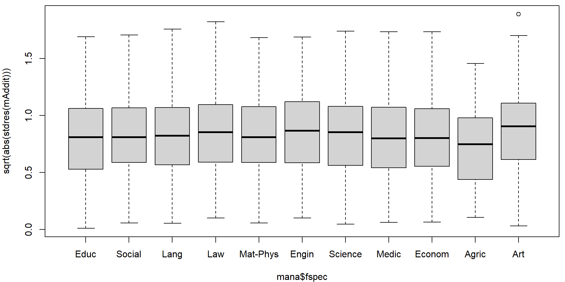
On first sight it seems that there are no issues with heteroscedasticity. However, if precise confidence intervals are desired it is better to be safe. We will use the sandwich estimate of the variance matrix to account for potential heteroscedasticity.
Generally, for the variance matrix of \(\widehat{\boldsymbol{\beta}}\) we have
\[
\mathsf{var} \left[ \left. \widehat{\boldsymbol{\beta}} \right|
\mathbb{X} \right]
=
\mathsf{var} \left[ \left. \left(\mathbb{X}^\top \mathbb{X}\right)^{-1}
\mathbb{X}^\top \mathbf{Y} \right| \mathbb{X} \right]
=
\left(\mathbb{X}^\top \mathbb{X}\right)^{-1} \mathbb{X}^\top
\mathsf{var} \left[ \left. \mathbf{Y} \right| \mathbb{X} \right]
\mathbb{X} \left(\mathbb{X}^\top \mathbb{X}\right)^{-1}.
\] Under homoscedasticity, \(\mathsf{var} \left[ \left. \mathbf{Y} \right|
\mathbb{X} \right] = \sigma^2 \mathbb{I}\) and the variance
estimator for \(\mathsf{var} \left[ \left.
\widehat{\boldsymbol{\beta}} \right| \mathbb{X} \right]\) is
\[
\widehat{\mathsf{var}} \left[ \left. \widehat{\boldsymbol{\beta}}
\right| \mathbb{X} \right]
=
\left(\mathbb{X}^\top \mathbb{X}\right)^{-1} \mathbb{X}^\top
\left[\widehat{\sigma}^2 \mathbb{I} \right]
\mathbb{X} \left(\mathbb{X}^\top \mathbb{X}\right)^{-1}
=
\widehat{\sigma}^2 \left(\mathbb{X}^\top \mathbb{X}\right)^{-1}.
\] Under heteroscedasticity, we consider
Heteroscedasticity-Consistent
covariance matrix estimator, which differs in the estimation of the
meat \(\mathsf{var} \left[ \left.
\mathbf{Y} \right| \mathbb{X} \right] = \mathsf{var} \left[ \left.
\boldsymbol{\varepsilon} \right| \mathbb{X} \right]\). Default
choice of type = "HC3" uses \[
\widehat{\mathsf{var}} \left[ \left. \mathbf{Y} \right| \mathbb{X}
\right]
=
\mathsf{diag} \left(U_i^2 / m_{ii}^2 \right),
\] where \(\mathbf{U} = \mathbf{Y} -
\widehat{\mathbf{Y}} = \mathbf{Y} - \mathbb{X} \left(\mathbb{X}^\top
\mathbb{X}\right)^{-1} \mathbb{X}^\top \mathbf{Y} = (\mathbb{I} -
\mathbb{H}) \mathbf{Y} = \mathbb{M} \mathbf{Y}\) are the
residuals.
library(sandwich)

### Estimate of the variance matrix of the regression coefficients
VHC <- vcovHC(mAddit, type = "HC3") # type changes the "meat"
VHC[1:5,1:5]
## (Intercept) fregionS fregionC fregionP fregionK
## (Intercept) 0.0002035881 -0.0001045279 -0.0001065979 -0.0001052227 -0.0001034781
## fregionS -0.0001045279 0.0001942935 0.0001020741 0.0001023074 0.0001011661
## fregionC -0.0001065979 0.0001020741 0.0002077926 0.0001022329 0.0001006027
## fregionP -0.0001052227 0.0001023074 0.0001022329 0.0004862487 0.0001010982
## fregionK -0.0001034781 0.0001011661 0.0001006027 0.0001010982 0.0004261994And we can compare the result with manually reconstructed estimate
X     <- model.matrix(mAddit)
Bread <- solve(t(X) %*% X) %*% t(X)
Meat  <- diag(residuals(mAddit)^2 / (1 - hatvalues(mAddit))^2)
(Bread %*% Meat %*% t(Bread))[1:5, 1:5]
## (Intercept) fregionS fregionC fregionP fregionK
## (Intercept) 0.0002035881 -0.0001045279 -0.0001065979 -0.0001052227 -0.0001034781
## fregionS -0.0001045279 0.0001942935 0.0001020741 0.0001023074 0.0001011661
## fregionC -0.0001065979 0.0001020741 0.0002077926 0.0001022329 0.0001006027
## fregionP -0.0001052227 0.0001023074 0.0001022329 0.0004862487 0.0001010982
## fregionK -0.0001034781 0.0001011661 0.0001006027 0.0001010982 0.0004261994all.equal(Bread %*% Meat %*% t(Bread), VHC)## [1] TRUEThis can be compared with the classical estimate of the variance covariance matrix - in the following, we only focus on some portion of the matrix multiplied by 10000.
10000*VHC[1:5, 1:5] ## (Intercept) fregionS fregionC fregionP fregionK
## (Intercept) 2.035881 -1.045279 -1.065979 -1.052227 -1.034781
## fregionS -1.045279 1.942935 1.020741 1.023074 1.011661
## fregionC -1.065979 1.020741 2.077926 1.022329 1.006027
## fregionP -1.052227 1.023074 1.022329 4.862487 1.010982
## fregionK -1.034781 1.011661 1.006027 1.010982 4.26199410000*vcov(mAddit)[1:5, 1:5]## (Intercept) fregionS fregionC fregionP fregionK
## (Intercept) 2.0495828 -1.0090753 -0.9704506 -0.9933825 -0.9449827
## fregionS -1.0090753 1.7808011 0.9400668 0.9440175 0.9342499
## fregionC -0.9704506 0.9400668 2.1167114 0.9436525 0.9366535
## fregionP -0.9933825 0.9440175 0.9436525 4.8251687 0.9394418
## fregionK -0.9449827 0.9342499 0.9366535 0.9394418 4.4005768Note, that some variance components are overestimated by the standard
estimate (function vcov()) and some others or
underestimated.
The inference then proceeds with the same point estimate \(\widehat{\boldsymbol{\beta}}\) but a
different vcovHC matrix instead of standard
vcov(). Classical summary table can be recalculated in the
following way:
coeftest(mAddit, vcov = VHC) # from library("lmtest")##
## t test of coefficients:
##
## Estimate Std. Error t value Pr(>|t|)
## (Intercept) 1.7761568 0.0142684 124.4816 < 2.2e-16 ***
## fregionS 0.0088705 0.0139389 0.6364 0.5245565
## fregionC -0.0133616 0.0144150 -0.9269 0.3540100
## fregionP 0.0200798 0.0220510 0.9106 0.3625455
## fregionK -0.0219780 0.0206446 -1.0646 0.2871117
## fregionU 0.0567816 0.0213933 2.6542 0.0079746 **
## fregionL 0.0238781 0.0141014 1.6933 0.0904561 .
## fregionH 0.0486074 0.0202311 2.4026 0.0163134 *
## fregionE 0.0798020 0.0216973 3.6780 0.0002375 ***
## fregionJ -0.0313805 0.0196311 -1.5985 0.1099897
## fregionB 0.0323584 0.0139521 2.3192 0.0204203 *
## fregionM 0.0258848 0.0242488 1.0675 0.2858099
## fregionZ 0.0165285 0.0183457 0.9009 0.3676588
## fregionT 0.0084599 0.0126113 0.6708 0.5023660
## fspecSocial -0.1507984 0.0128745 -11.7129 < 2.2e-16 ***
## fspecLang -0.2638676 0.0168792 -15.6327 < 2.2e-16 ***
## fspecLaw -0.1502042 0.0152848 -9.8271 < 2.2e-16 ***
## fspecMat-Phys -0.2219191 0.0188825 -11.7526 < 2.2e-16 ***
## fspecEngin -0.1775146 0.0141988 -12.5021 < 2.2e-16 ***
## fspecScience -0.1041070 0.0143710 -7.2442 4.988e-13 ***
## fspecMedic -0.1436849 0.0141332 -10.1665 < 2.2e-16 ***
## fspecEconom -0.1675115 0.0128221 -13.0643 < 2.2e-16 ***
## fspecAgric -0.0711497 0.0271456 -2.6210 0.0087917 **
## fspecArt -0.1552720 0.0222920 -6.9654 3.684e-12 ***
## ---
## Signif. codes: 0 '***' 0.001 '**' 0.01 '*' 0.05 '.' 0.1 ' ' 1Unfortunately, function predict.lm is not as flexible
and confidence intervals need to be computed manually
newdata <- data.frame(fregion = "A",
                      fspec = levels(mana$fspec),
                      avg.mark = 0)
# predict no sandwich
pred_vcov <- predict(mAddit, newdata = newdata, interval = "confidence")

# predict with sandwich (manually)
L <- model.matrix(mAddit, data = newdata)
se.fit <- sqrt(diag(L %*% VHC %*% t(L)))
pred_VHC <- matrix(NA, nrow = nrow(L), ncol = 3)
pred_VHC[,1] <- L %*% coef(mAddit)
pred_VHC[,2] <- pred_VHC[,1] - se.fit * qt(0.975, df = mAddit$df.residual)
pred_VHC[,3] <- pred_VHC[,1] + se.fit * qt(0.975, df = mAddit$df.residual)
colnames(pred_VHC) <- c("fit", "lwr", "upr")
rownames(pred_VHC) <- rownames(pred_vcov)

all.equal(pred_vcov[,"fit"], pred_VHC[,"fit"])
## [1] TRUEall.equal(pred_vcov[,"lwr"], pred_VHC[,"lwr"])## [1] "Mean relative difference: 0.001029055"all.equal(pred_vcov[,"upr"], pred_VHC[,"upr"])## [1] "Mean relative difference: 0.0009898677"par(mfrow = c(1,1), mar = c(4,4,0.5,0.5))
plot(x = 1:nlevels(mana$fspec), y = pred_vcov[,"fit"],
xlab = "Specialization", ylab = "Expected average mark, Prague region",
xaxt = "n", ylim = range(pred_vcov, pred_VHC),
col = "red4", pch = 16, cex = 2)
axis(1, at = 1:nlevels(mana$fspec), labels = levels(mana$fspec))
arrows(x0 = 1:nlevels(mana$fspec), y0 = pred_vcov[,"lwr"], y1 = pred_vcov[,"upr"],
angle = 80, lwd = 2, col = "red", code = 3)
arrows(x0 = 1:nlevels(mana$fspec), y0 = pred_VHC[,"lwr"], y1 = pred_VHC[,"upr"],
angle = 80, lwd = 2, col = "navyblue", code = 3)
legend("top", legend = c("vcov()", "vcovHC(type = 'HC3')"),
ncol = 2, bty = "n", col = c("red", "navyblue"), lwd = 2)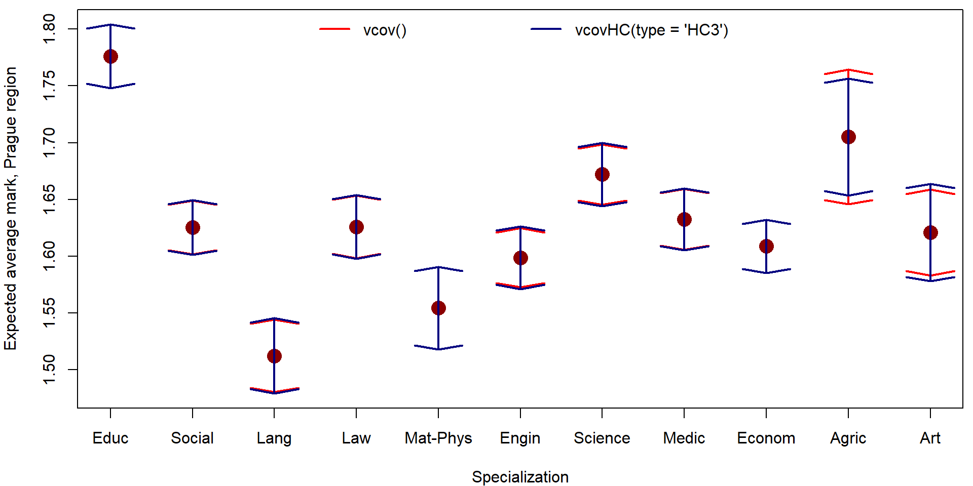
3. Motorcycle example with bounds
We will simply take the Motorcycle data from previous
exercise fitted with splines and add the confidence bands corrected for
heterescedasticity via sandwich estimator. First, we fit the splines
model again:
data(Motorcycle, package = "mffSM")
head(Motorcycle)
## time haccel
## 1 2.4 0.0
## 2 2.6 -1.3
## 3 3.2 -2.7
## 4 3.6 0.0
## 5 4.0 -2.7
## 6 6.2 -2.7### Choice of knots
library(splines)
knots <- c(0, 11, 12, 13, 20, 30, 32, 34, 40, 50, 70)
(inner <- knots[-c(1, length(knots))]) # inner knots ## [1] 11 12 13 20 30 32 34 40 50(bound <- knots[c(1, length(knots))]) # boundary knots ## [1] 0 70### B-splines of degree 3
DEGREE <- 3 # piecewise cubic
xgrid <- seq(0, 70, length = 500)
Bgrid <- bs(xgrid, knots = inner, Boundary.knots = bound, degree = DEGREE, intercept = FALSE)
m <- lm(haccel ~ bs(time, knots = inner, Boundary.knots = bound,
degree = DEGREE, intercept = FALSE), data = Motorcycle)
# change the names of the coefficients
names(m$coefficients)[-1] <- paste("B", 1:ncol(Bgrid))
summary(m)##
## Call:
## lm(formula = haccel ~ bs(time, knots = inner, Boundary.knots = bound,
## degree = DEGREE, intercept = FALSE), data = Motorcycle)
##
## Residuals:
## Min 1Q Median 3Q Max
## -71.857 -11.740 -0.268 10.356 55.249
##
## Coefficients:
## Estimate Std. Error t value Pr(>|t|)
## (Intercept) -11.614 83.252 -0.140 0.8893
## B 1 24.064 161.970 0.149 0.8821
## B 2 -2.374 57.835 -0.041 0.9673
## B 3 14.598 93.327 0.156 0.8760
## B 4 17.729 80.496 0.220 0.8261
## B 5 -225.669 88.698 -2.544 0.0122 *
## B 6 28.960 82.780 0.350 0.7271
## B 7 64.862 84.773 0.765 0.4457
## B 8 16.716 83.997 0.199 0.8426
## B 9 24.223 85.172 0.284 0.7766
## B 10 -23.335 91.337 -0.255 0.7988
## B 11 69.869 105.918 0.660 0.5107
## B 12 -81.454 112.465 -0.724 0.4703
## ---
## Signif. codes: 0 '***' 0.001 '**' 0.01 '*' 0.05 '.' 0.1 ' ' 1
##
## Residual standard error: 22.61 on 120 degrees of freedom
## Multiple R-squared: 0.8009, Adjusted R-squared: 0.781
## F-statistic: 40.23 on 12 and 120 DF, p-value: < 2.2e-16Let us examine the issues with heteroscedasticity and confirm them by tests:
par(mfrow = c(1,2), mar = c(4,4,2,1))
plot(abs(fitted(m)), sqrt(abs(stdres(m))),
     main = "Abs(fitted)",
     lwd=2, col="blue4", bg="skyblue", pch=21)
lines(lowess(abs(fitted(m)), sqrt(abs(stdres(m)))), col="red", lwd=3)

plot(Motorcycle$time, sqrt(abs(stdres(m))),
     main = "Time",
     lwd=2, col="blue4", bg="skyblue", pch=21)
lines(lowess(Motorcycle$time, sqrt(abs(stdres(m)))), col="red", lwd=3)
### Koenker's studentized version of Breusch-Pagan tests (robust to non-normality)
bptest(m, varformula = ~fitted(m))     # monotone change with fitted values ~ E[Y|X=x]
##
## studentized Breusch-Pagan test
##
## data: m
## BP = 0.0046535, df = 1, p-value = 0.9456bptest(m, varformula = ~fitted(m) + I(fitted(m)^2)) # quadratic change with ##
## studentized Breusch-Pagan test
##
## data: m
## BP = 1.1581, df = 2, p-value = 0.5604bptest(m, varformula = ~I(Motorcycle$time > 15)) # change at time 15 ##
## studentized Breusch-Pagan test
##
## data: m
## BP = 10.175, df = 1, p-value = 0.001424bptest(m, varformula = ~Motorcycle$time + I(Motorcycle$time^2)) # quadratic change with time##
## studentized Breusch-Pagan test
##
## data: m
## BP = 15.306, df = 2, p-value = 0.0004745Confidence and prediction intervals with the plain
vcov() estimator
newdata <- data.frame(time = xgrid, haccel = 0)
pred_around <- predict(m, newdata = newdata, interval = "confidence", se.fit = TRUE)
pred_pred <- predict(m, newdata = newdata, interval = "prediction")
qfor <- sqrt(m$rank * qf(0.95, df1 = m$rank, df2 = m$df.residual))
pred_for <- data.frame(fit = pred_around$fit[,"fit"],
                       lwr = pred_around$fit[,"fit"] - qfor * pred_around$se.fit,
                       upr = pred_around$fit[,"fit"] + qfor * pred_around$se.fit)

par(mfrow = c(1,1), mar = c(4,4,2,1))
plot(haccel ~ time, data = Motorcycle, pch = 21, bg = "orange", col = "red3",
     main = "Fitted B-spline curve, HOMOscedastic model",
     xlab = "Time [ms]", ylab = "Head acceleration [g]",
     ylim = c(-150, 100))
lines(xgrid, pred_around$fit[, "fit"], lwd = 2, col = "darkviolet")
# confidence intervals - AROUND the regression curve
lines(xgrid, pred_around$fit[, "lwr"], lwd = 2, lty = 2, col = "skyblue")
lines(xgrid, pred_around$fit[, "upr"], lwd = 2, lty = 2, col = "skyblue")
# confidence intervals - FOR the regression curve
lines(xgrid, pred_for[, "lwr"], lwd = 2, lty = 3, col = "blue")
lines(xgrid, pred_for[, "upr"], lwd = 2, lty = 3, col = "blue")
# prediction intervals
lines(xgrid, pred_pred[, "lwr"], lwd = 2, lty = 4, col = "navyblue")
lines(xgrid, pred_pred[, "upr"], lwd = 2, lty = 4, col = "navyblue")

legend(40, -80, legend = c("Fit", "Around", "For", "Prediction"),
       col = c("darkviolet", "skyblue", "blue", "navyblue"), lwd = 2, lty = 1:4)
Confidence and prediction intervals with the sandwich estimator
VHC <- vcovHC(m, type = "HC3")
L <- model.matrix(m, data = newdata)
se.fit <- sqrt(diag(L %*% VHC %*% t(L)))
VHC_around <- data.frame(fit = L %*% coef(m))
VHC_around$lwr <- VHC_around$fit - se.fit * qt(0.975, df = m$df.residual)
VHC_around$upr <- VHC_around$fit + se.fit * qt(0.975, df = m$df.residual)

qfor <- sqrt(m$rank * qf(0.95, df1 = m$rank, df2 = m$df.residual))
VHC_for <- data.frame(fit = VHC_around$fit,
                      lwr = VHC_around$fit - qfor * se.fit,
                      upr = VHC_around$fit + qfor * se.fit)

# Prediction intervals require the estimate for sigma_new^2
# should be different from sigma^2
se_vs_pred <- se.fit / pred_around$se.fit           # how differs the variability for E[Y|X=x]
sigma <- sqrt(sum(residuals(m)^2) / m$df.residual)  # sigma in homoscedastic model
flexible_sigma <- se_vs_pred * sigma                # multiply sigma proportionally

pred.fit <- sqrt(flexible_sigma^2 + diag(L %*% VHC %*% t(L)))
VHC_pred <- data.frame(fit = L %*% coef(m))
VHC_pred$lwr <- VHC_pred$fit - pred.fit * qt(0.975, df = m$df.residual)
VHC_pred$upr <- VHC_pred$fit + pred.fit * qt(0.975, df = m$df.residual)


par(mfrow = c(1,1), mar = c(4,4,2,1))
plot(haccel ~ time, data = Motorcycle, pch = 21, bg = "orange", col = "red3",
     main = "Fitted B-spline curve, HETEROscedastic model",
     xlab = "Time [ms]", ylab = "Head acceleration [g]",
     ylim = c(-150, 100))
lines(xgrid, VHC_around[, "fit"], lwd = 2, col = "darkviolet")
# confidence intervals - AROUND the regression curve
lines(xgrid, VHC_around[, "lwr"], lwd = 2, lty = 2, col = "orange")
lines(xgrid, VHC_around[, "upr"], lwd = 2, lty = 2, col = "orange")
# confidence intervals - FOR the regression curve
lines(xgrid, VHC_for[, "lwr"], lwd = 2, lty = 3, col = "red")
lines(xgrid, VHC_for[, "upr"], lwd = 2, lty = 3, col = "red")
# prediction intervals
lines(xgrid, VHC_pred[, "lwr"], lwd = 2, lty = 4, col = "red4")
lines(xgrid, VHC_pred[, "upr"], lwd = 2, lty = 4, col = "red4")

legend(40, -80, legend = c("Fit", "Around", "For", "Prediction"),
       col = c("darkviolet", "orange", "red", "red4"), lwd = 2, lty = 1:4)
Compare the bands between each other:
par(mfrow = c(1,1), mar = c(4,4,2,1))
# confidence intervals - AROUND the regression curve
plot(haccel ~ time, data = Motorcycle, pch = 21, bg = "orange", col = "red3",
     main = "AROUND bands",
     xlab = "Time [ms]", ylab = "Head acceleration [g]",
     ylim = c(-150, 100))
lines(xgrid, VHC_around[, "fit"], lwd = 2, col = "darkviolet")
lines(xgrid, pred_around$fit[, "lwr"], lwd = 2, lty = 2, col = "skyblue")
lines(xgrid, pred_around$fit[, "upr"], lwd = 2, lty = 2, col = "skyblue")
lines(xgrid, VHC_around[, "lwr"], lwd = 2, lty = 2, col = "orange")
lines(xgrid, VHC_around[, "upr"], lwd = 2, lty = 2, col = "orange")
legend(40, -80, legend = c("vcov", "sandwich"), col = c("skyblue", "orange"), lwd = 2, lty = 2)
# confidence intervals - FOR the regression curve
plot(haccel ~ time, data = Motorcycle, pch = 21, bg = "orange", col = "red3",
     main = "FOR bands",
     xlab = "Time [ms]", ylab = "Head acceleration [g]",
     ylim = c(-150, 100))
lines(xgrid, VHC_around[, "fit"], lwd = 2, col = "darkviolet")
lines(xgrid, pred_for[, "lwr"], lwd = 2, lty = 3, col = "blue")
lines(xgrid, pred_for[, "upr"], lwd = 2, lty = 3, col = "blue")
lines(xgrid, VHC_for[, "lwr"], lwd = 2, lty = 3, col = "red")
lines(xgrid, VHC_for[, "upr"], lwd = 2, lty = 3, col = "red")
legend(40, -80, legend = c("vcov", "sandwich"), col = c("blue", "red"), lwd = 2, lty = 3)
# prediction intervals
plot(haccel ~ time, data = Motorcycle, pch = 21, bg = "orange", col = "red3",
     main = "Prediction bands",
     xlab = "Time [ms]", ylab = "Head acceleration [g]",
     ylim = c(-150, 100))
lines(xgrid, VHC_around[, "fit"], lwd = 2, col = "darkviolet")
lines(xgrid, pred_pred[, "lwr"], lwd = 2, lty = 4, col = "navyblue")
lines(xgrid, pred_pred[, "upr"], lwd = 2, lty = 4, col = "navyblue")
lines(xgrid, VHC_pred[, "lwr"], lwd = 2, lty = 4, col = "red4")
lines(xgrid, VHC_pred[, "upr"], lwd = 2, lty = 4, col = "red4")
legend(40, -80, legend = c("vcov", "sandwich"), col = c("navyblue", "red4"), lwd = 2, lty = 4)