Next: Boundary Conditions
Up: Formulation of the Problem
Previous: Formulation of the Problem
In this section we will formulate the initial-boundary value problem for
considered inviscid-viscous flows. It means that the system of equations
(14) will be completed by some boundary and initial conditions.
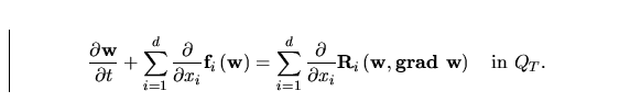
Firstly, we rewrite (14) in the so-called
conservative form.
In problems that will be numerically solved we will neglect the heat
sources (i.e. q=0) and the volume forces ( i.e.  ). We define
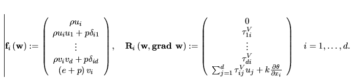
the state vector
). We define
the state vector
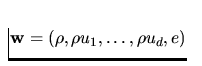 and rewrite (14) in the
following way:
and rewrite (14) in the
following way:
|  |
(14) |
Here
The functions  are called the inviscid
Euler fluxes and
are called the inviscid
Euler fluxes and 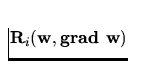 are called
the viscous fluxes.
are called
the viscous fluxes.
The system (15) gives the conservative form of the complete
Navier-Stokes equations for viscous fluids. In the case of inviscid
fluids  and, hence,
  Therefore,
the conservative form of the Euler equations can be written in the form
Therefore,
the conservative form of the Euler equations can be written in the form
|  |
(15) |
Moreover, the state equations should be added to close the system
(15) or (17). Using (9) we get
|  |
(16) |
Next: Boundary Conditions
Up: Formulation of the Problem
Previous: Formulation of the Problem
Vit Dolejsi
12/17/1998